文章目录(Table of Contents)
简介
这里会介绍关于因子分析的实战, 我们会去实际分析一下关于人格的数据集. 下面是一些参考链接, 主要内容参考自第一个链接.
- 因子分析实战: https://www.datacamp.com/community/tutorials/introduction-factor-analysis
- 数据集介绍: https://vincentarelbundock.github.io/Rdatasets/doc/psych/bfi.html
- 数据集下载: https://vincentarelbundock.github.io/Rdatasets/datasets.html
- factor_analyzer网站: https://github.com/EducationalTestingService/factor_analyzer
因子分析实战
数据集简单介绍
使用了bfi2010的数据集, 这个数据集收集了2800个人关于人格的25个问题, 这些问题下面举几个例子(详细的介绍看上面的链接数据集介绍)
- Am indifferent to the feelings of others. (对别人的感受漠不关心)
- Inquire about others‘ well-being. (询问他人是否幸福)
- Know how to comfort others. (知道如何让安慰别人)
- Love children. (喜欢孩子)
- Make people feel at ease. (让人感到轻松)
- Am exacting in my work. (对工作热情)
- ... ...
同时, 这些特征是与5个隐藏特征有关, 这5个特征就是5大人格特征: Big Five Model is widely used nowadays, the five factors include: neuroticism, extraversion, openness to experience, agreeableness and conscientiousness.
关于特征之间的对应关系如下所示(之后的因子分析也是可以证明这个的):
- agree=c(“-A1”,“A2”,“A3”,“A4”,“A5”) => 认同性
- conscientious=c(“C1”,“C2”,“C3”,“-C4”,“-C5”) => 勤奋的, 责任感
- extraversion=c(“-E1”,“-E2”,“E3”,“E4”,“E5”) => 外向的
- neuroticism=c(“N1”,“N2”,“N3”,“N4”,“N5”) => 神经质, 不稳定性
- openness = c(“O1”,“-O2”,“O3”,“O4”,“-O5”) => 开放性
其实我们是不知道这种对应关系的, 这5大人格相当于是5个隐藏变量, 这些隐藏变量会导致我们观测的变化, 所以我们相当于想要通过因子分析来找到这25个变量后面的隐藏变量. 下面就进行因子分析.
因子分析实做
导入需要使用的库
- # Import required libraries
- import numpy as np
- import pandas as pd
- from factor_analyzer import FactorAnalyzer
- import matplotlib.pyplot as plt
导入数据并做处理
接着导入数据, 并做一下简单的数据处理, 去除一些缺失数据.
- df= pd.read_csv("bfi.csv")
- # Dropping unnecessary columns
- df.drop(['Unnamed: 0', 'gender', 'education', 'age'],axis=1,inplace=True)
- # Dropping missing values rows
- df.dropna(inplace=True)
- df.head()
处理完毕之后数据如下所示
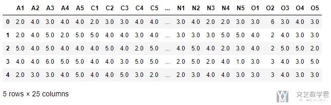
同时数据的大小为, 2436*25.
充分性测试(Adequacy Test)
在做因子分析之前, 我们需要先做充分性检测, 就是数据集中是否能找到这些factor, 我们可以使用下面的两种方式进行寻找.
- Bartlett's Test
- Kaiser-Meyer-Olkin Test
Bartlett's test of sphericity 是用来检测观察到的变量之间是否关联, 如果检测结果在统计学上不显著, 就不能采用因子分析.
- from factor_analyzer.factor_analyzer import calculate_bartlett_sphericity
- chi_square_value,p_value=calculate_bartlett_sphericity(df)
- chi_square_value, p_value
- """
- (18170.966350869257, 0.0)
- """
p-value=0, 表明观察到的相关矩阵不是一个identity matrix.
Kaiser-Meyer-Olkin (KMO) Test measures the suitability of data for factor analysis. It determines the adequacy for each observed variable and for the complete model. KMO estimates the proportion of variance among all the observed variable. Lower proportion id more suitable for factor analysis. KMO values range between 0 and 1. Value of KMO less than 0.6 is considered inadequate.(就是kmo值要大于0.6)
- from factor_analyzer.factor_analyzer import calculate_kmo
- kmo_all,kmo_model=calculate_kmo(df)
- print(kmo_model)
- """
- 0.848539722194922
- """
选择合适的因子个数
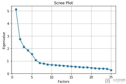
在这个问题下, 虽然我们知道了选择5个因子是最合适的, 但是我们也要做一步这个, 正常的时候我们是不会提前知道因子选择的个数的. 我们就是计算相关矩阵的特征值, 接着进行排序.
- # Create factor analysis object and perform factor analysis
- fa = FactorAnalyzer(25, rotation=None)
- fa.fit(df)
- # Check Eigenvalues
- ev, v = fa.get_eigenvalues()
接着我们将其进行可视化操作:
- # Create scree plot using matplotlib
- plt.scatter(range(1,df.shape[1]+1),ev)
- plt.plot(range(1,df.shape[1]+1),ev)
- plt.title('Scree Plot')
- plt.xlabel('Factors')
- plt.ylabel('Eigenvalue')
- plt.grid()
- plt.show()
进行因子分析
我们对数据进行因子分析, 找5个隐藏因子.
- fa = FactorAnalyzer(5, rotation="varimax")
- fa.fit(df)
- """
- FactorAnalyzer(bounds=(0.005, 1), impute='median', is_corr_matrix=False,
- method='minres', n_factors=5, rotation='varimax',
- rotation_kwargs={}, use_smc=True)
- """
接着我们输出因子的系数
- # 25*5(变量个数*因子个数)
- fa.loadings_
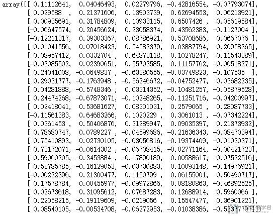
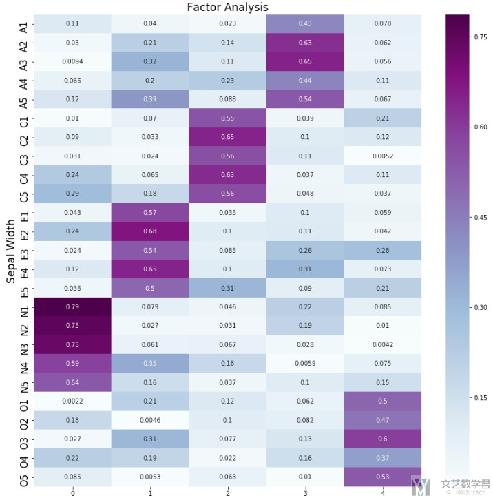
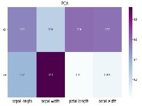
可以看到直接输出系数不是很直观, 看不出每一个隐藏变量与哪些变量的关系比较大. 我们将其可视化展示, 为了显示效果, 我们将其求绝对值.
- import seaborn as sns
- df_cm = pd.DataFrame(np.abs(fa.loadings_), index=df.columns)
- plt.figure(figsize = (14,14))
- ax = sns.heatmap(df_cm, annot=True, cmap="BuPu")
- # 设置y轴的字体的大小
- ax.yaxis.set_tick_params(labelsize=15)
- plt.title('Factor Analysis', fontsize='xx-large')
- # Set y-axis label
- plt.ylabel('Sepal Width', fontsize='xx-large')
- plt.savefig('factorAnalysis.png', dpi=500)
最终的效果如下图所示, 可以看到每一个隐变量都是与5个观测变量由较大的关系, 这个是与我们之前分析的是一样的.
转换为新的变量
最后, 就是当我们知道使用新的5个变量比较合适之后, 我们将原始的数据都转换为5个新的特征, 转换的方式如下所示:
- fa.transform(df)
最后输出的大小是2436*5, 也就是每一个数据都有5个特征.
代码仓库
Github仓库Notebook: PCA(主成分分析)+FA(因子分析)
- 微信公众号
- 关注微信公众号
-

- QQ群
- 我们的QQ群号
-


评论