文章目录(Table of Contents)
前言
这一篇记录一下关于Python在科学运算上的一些操作,方便查询。之后会不定期补充。
矩阵运算
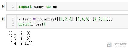
- import numpy as np
- x_test = np.array([[1,2,3],[3,4,6],[4,7,11]])
- print(x_test)
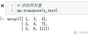
矩阵转置
- # 求矩阵转置
- np.transpose(x_test)
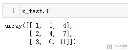
当然,也可以通过下面方式求转置
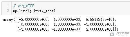
矩阵求逆
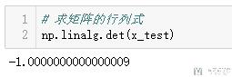
矩阵求行列式
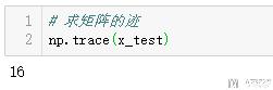
矩阵求迹
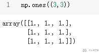
生成全1矩阵
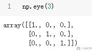
生成对角矩阵
特征值与特征向量
- # 求矩阵的特征值与特征向量
- w, v = np.linalg.eig(x_test)
- print("Eigenvalues : \n{}".format(w)) # 特征值
- print("Eigenvectors : \n{}".format(v)) # 特征向量
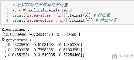
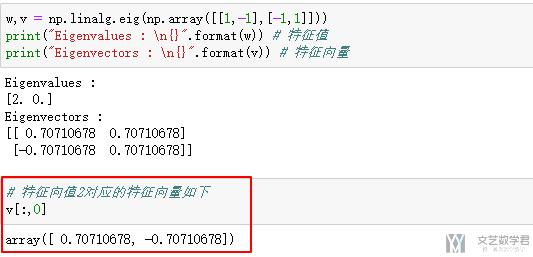
特别要注意的是,特征值w[i]对应的特征向量为v[:,i],我们看一下下面的例子:
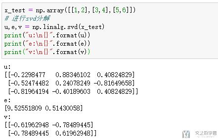
SVD分解
- x_test = np.array([[1,2],[3,4],[5,6]])
- # 进行svd分解
- u,e,v = np.linalg.svd(x_test)
- print("u:\n{}".format(u))
- print("e:\n{}".format(e))
- print("v:\n{}".format(v))
- # 将e矩阵补齐
- e_n = np.zeros([3,2])
- for i in range(2):
- e_n[i][i] = e[i]
- print("u:\n{}".format(u))
- print("e_n:\n{}".format(e_n))
- print("v:\n{}".format(v))
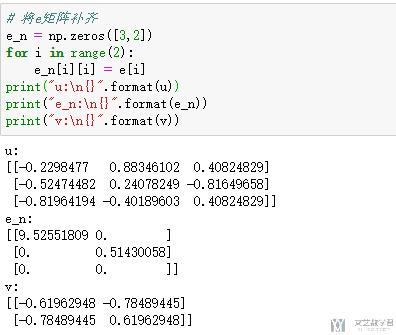
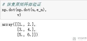
下面验证一下SVD分解的结果是否正确
- # 恢复原矩阵做验证
- np.dot(np.dot(u,e_n),
- v)
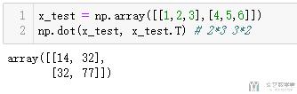
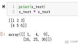
矩阵乘法
- x_test = np.array([[1,2,3],[4,5,6]])
- np.dot(x_test, x_test.T) # 2*3 3*2
若直接使用乘法, 只是元素间的两两相乘;
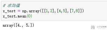
统计相关
均值, 方差, 标准差
- # 求均值
- x_test = np.array([[1,2],[4,5],[7,8]])
- x_test.mean(0)
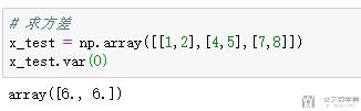
- # 求方差
- x_test = np.array([[1,2],[4,5],[7,8]])
- x_test.var(0)
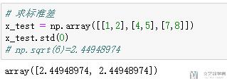
- # 求标准差
- x_test = np.array([[1,2],[4,5],[7,8]])
- x_test.std(0)
- # np.sqrt(6)=2.44948974
协方差矩阵
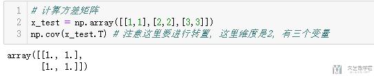
- # 计算方差矩阵
- x_test = np.array([[1,1],[2,2],[3,3]])
- np.cov(x_test.T) # 注意这里要进行转置, 这里维度是2, 有三个变量
相关系数矩阵
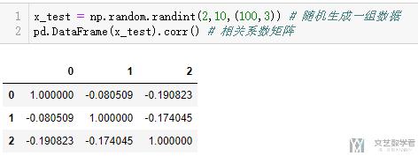
- x_test = np.random.randint(2,10,(100,3)) # 随机生成一组数据
- pd.DataFrame(x_test).corr() # 相关系数矩阵
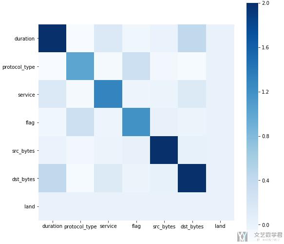
协方差矩阵与相关系数矩阵可视化
有时候,我们会把相关系数矩阵绘制成heatmap,这样可以更加直观的显示出效果;
- import seaborn as sns
- import matplotlib.pyplot as plt
- %matplotlib inline
- # 这里数据集是我之前的一个数据, 具体使用的时候进行修改即可
- dfData = data_guess.iloc[:,:7].cov()
- plt.subplots(figsize=(9, 9)) # 设置画面大小
- sns.heatmap(dfData,square=True, cmap="Blues")
上面代码的绘制效果如下所示:
数据预处理
- from sklearn import preprocessing
首先介绍一下标准化的几个式子,下面截图来自知乎:
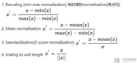
一般把第一种叫做归一化,第三种叫做标准化。关于详细的介绍,可以查看知乎的链接,标准化和归一化什么区别?
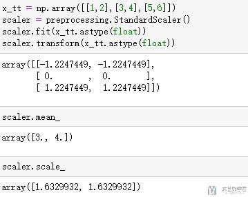
StandardScaler
在sklearn中,可以有两种方式进行实现数据的标准化,分别是使用函数scale和使用类StandardScaler(),下面分别来看一下:
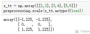
使用scale进行计算:
- x_tt = np.array([[1,2],[3,4],[5,6]])
- preprocessing.scale(x_tt.astype(float))
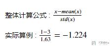
我们看一下实际的计算结果
当然,我们可以使用StandardScaler()来进行计算,使用这种方式可以查看每一维特征的均值和方差。
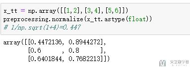
Normalize
计算的步骤我用注释的方法写在了代码下面。
- x_tt = np.array([[1,2],[3,4],[5,6]])
- preprocessing.normalize(x_tt.astype(float))
- # 1/np.sqrt(1+4)=0.447
Label的生成
有的时候我们的数据集中的label是string类型的, 例如是"paris", "paris", "tokyo", "amsterdam", 但是实际在训练的时候, 我们需要将其转换为long类型的. 这个时候就可以使用sklearn.preprocessing.LabelEncoder. 下面看一下简单的用法:
- from sklearn import preprocessing
- le = preprocessing.LabelEncoder()
接着对于我们要转换的数据, 使用fit函数.
- le.fit(["paris", "paris", "tokyo", "amsterdam"])
- # >> LabelEncoder()
我们可以查看有多少种不同的classes.
- list(le.classes_)
- # >> ['amsterdam', 'paris', 'tokyo']
接着我们可以对原始数据进行转换. 将string类型的label转换为int类型的.
- le.transform(["tokyo", "tokyo", "paris"])
- # >> array([2, 2, 1]...)
同时我们也可以逆向转换, 将index再转换为string类型的label.
- list(le.inverse_transform([2, 2, 1]))
- # >> ['tokyo', 'tokyo', 'paris']
离散变量变为标号(可以不用看, 使用上面的LabelEncoder代替)
有的时候,我们会将离散变量转为标号的表示(大部分情况会变为one-hot编码,转为one-hot的方式在下面介绍)
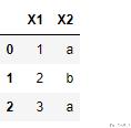
首先生成我们需要的测试数据:
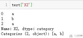
- test = pd.DataFrame(np.array([[1,'a'],[2,'b'],[3,'a']]),columns=['X1','X2'])
- test
我们首先看一下X2的类型,可以看到是object,我们可以将其转换为category.
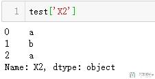
- test['X2']=test['X2'].astype('category')
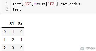
接着我们就可以将其变为数字标号了。
- test['X2']=test['X2'].cat.codes
- test
下面放一下完整的片段
- test = pd.DataFrame(np.array([[1,'a'],[2,'b'],[3,'a']]),columns=['X1','X2'])
- test = test.astype('category')
- for i in test.columns:
- test[i] = test[i].cat.codes
One-hot编码
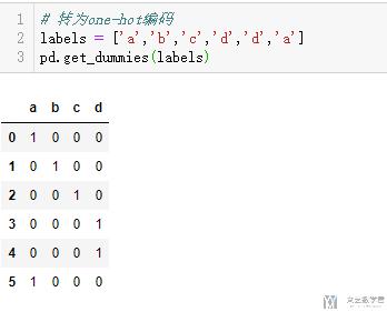
对于离散得特征,我们通常会将他们转换为one-hot编码得形式,我们可以使用pandas完成相关得操作。下面是一个简单得例子。
- # 转为one-hot编码
- labels = ['a','b','c','d','d','a']
- pd.get_dummies(labels)
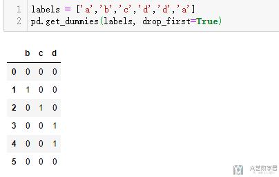
我们也是可以设置drop_first=True来是的N维的特征使用N-1维来进行表示. 我们来看一个简单的例子. 比如说, 现在一个离散特征有三个取值, a, b, c. 那么我们只需要二维就可以表示 (二维应该可以表示2^2不同的组合, 但是这里不同有多个1同时出现).
- a: [0, 0]
- b: [1, 0]
- c: [0, 1]
下面我们实际来举一个例子.
- labels = ['a','b','c','d','d','a']
- pd.get_dummies(labels, drop_first=True)
于是我们得到了下面的结果, 一共有a,b,c,d四种组合, 这里用三维的one-hot向量进行表示:
关于One-hot的一点进阶说明
在使用pd.get_dummies将离散数据转换为one-hot的时候, 若原始数据集中包含其他类型的数据, 是否得到保留, 所以我们可以对整个数据直接进行pd.get_dummies, 我们看下面的例子.
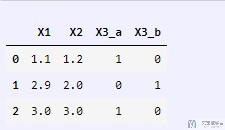
在a中, X1和X2是连续型的, X3是离散型的, 我们只需要对X3进行转换.
- a = pd.DataFrame(np.array([[1.1,1.2,'a'],[2.9,2.0,'b'],[3,3,'a']]),columns=['X1','X2','X3'])
- a['X1'] = a['X1'].astype(float)
- a['X2'] = a['X2'].astype(float)
- pd.get_dummies(a)
最终的结果如下所示, 可以看到X1和X2是不会改变的.
抽样与乱序
有的时候,我们需要在样本中进行抽样,或是打乱样本的顺序,我们可以使用如下的方式进行操作。
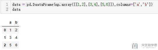
我们使用下面的数据进行一下实验:
- data = pd.DaataFrame(np.array([[1,2],[3,4],[5,6]]),columns=['a','b'])
- data
抽样
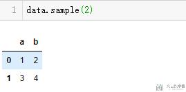
我们可以抽指定个数的样本:
- data.sample(2)
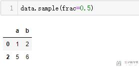
也可以抽取指定比例的样本:
乱序
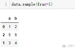
想要进行打乱样本的顺序,我们只需要进行比例为1的抽样即可:
- data.sample(frac=1)
乱序之后, 我们还需要对index进行重新的排序, 方法如下所示:
- test.reset_index(drop=True, inplace=True)
划分训练集和测试集
我们使用sklearn.model_selection.train_test_split来进行训练集和测试集的划分. 下面是简单的使用.
- import numpy as np
- from sklearn.model_selection import train_test_split
- X_train, X_test, y_train, y_test = train_test_split(X, y, test_size=0.33, random_state=42)
- 微信公众号
- 关注微信公众号
-

- QQ群
- 我们的QQ群号
-


评论