文章目录(Table of Contents)
简介
这一部分简单介绍一下Recurrent Neural Network(RNN)的内容。主要会包括普通RNN(包括deeper的情况下和Bidirectional RNN), LSTM, GRU介绍。并简单介绍一下计算的方式,简单使用PyTorch进行实验。这一部分还是主要是为了熟悉RNN的基本内容。
参考资料
把参考资料放在最前面,后面可能讲的不怎么好,可以直接从这里查看原文。
关于RNN基础介绍资料 : Recurrent Neural Networks Tutorial, Part 1 – Introduction to RNNs
关于LSTM和GRU介绍资料 : Recurrent Neural Network Tutorial, Part 4 – Implementing a GRU/LSTM RNN with Python and Theano
详细介绍LSTM的资料(这里介绍的LSTM很详细, 十分建议自己看一遍, 他一步一步教你LSTM是如何操作的) : Understanding LSTM Networks
BPTT的推导(这是一个推导的pdf, 内容很详细) : Gradients for an RNN
一些RNN的应用介绍(这里也会有RNN的大概的介绍, 但是更多的是应用的介绍) : The Unreasonable Effectiveness of Recurrent Neural Networks
RNN想要解决的问题
传统网络的问题
下面三个是传统的RNN的局限所在。
- The idea behind RNNs is to make use of sequential information. In a traditional neural network we assume that all inputs (and outputs) are independent of each other. But for many tasks that's a very bad idea.(在传统的网络中, 我们假设input内部相互之间是没有关系的, 或是output的内部之间也是没有相互关系的)
- 同时input的长度需要时固定长度的。
- 同时, 我们输入的input相同, output也会是相同的。但有时我们需要input相同但是output是不同的。例如下面的例子
-
- 下面两个句子, 有着相同的word, 如果用 word of bag表示是一样的;
- 但是这两句话表达的情感是不一样的, 如果使用Fully Connection Network上面是无法分类的.(即相同的input, 但是output不同)
- White blood cells destroying an infection. -> Positive
- An infection destroying white blood cells. -> Negative
解决的思路
于是,我们希望我们的网络是有记忆的,这样记住每次input的顺序,这样即使input是一样的,但是顺序不同,output就也是不同的。
典型的RNN结构
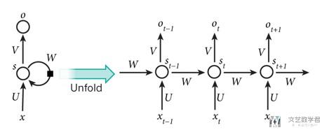
下面是一个典型的RNN网络的结构。A recurrent neural network can be thought of as multiple copies of the same network, each passing a message to a successor.
下图可以理解为,我们将RNN从时间上进行展开。
Simple RNN
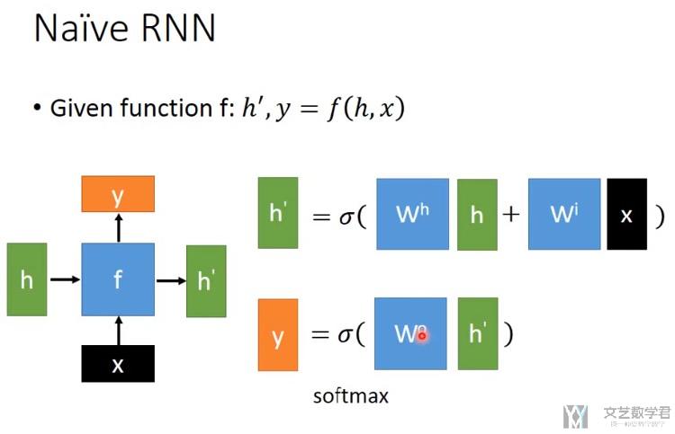
下面介绍一下最简单的RNN是如何进行计算的。如下图所示:
- input : 输入为X
- h表示hidden state,相当于我们所说的记忆。(我们可以看到hidden每次都会被抹去, 之后LSTM会有所改进)
- output是y,y的计算会与输入x与记忆h有关
我们看一下RNN展开之后的样子,如下所示。其实需要计算的系数就是上面的W_i和W_h,下面的图片只不过是在各个时间段展开,这样就可以使得input的长度是变长的。
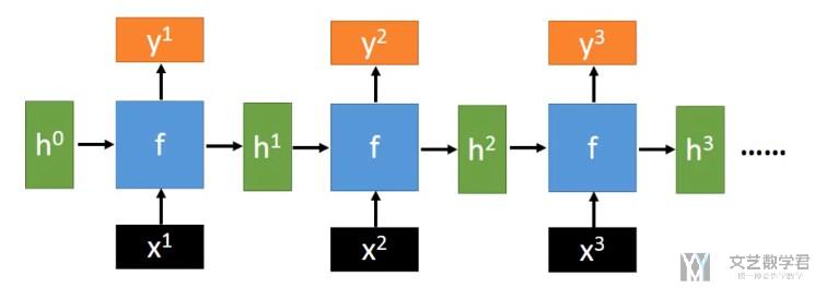
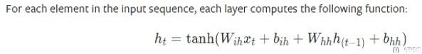
整体的一个计算的式子如下所示,其中W_ih表示上图的W_i(也就是input乘的系数), W_hh表示上图的W_h(也就是hidden state的系数)
RNN can be deep
当然,RNN网络可以变得更深,我们来简单看一个例子。
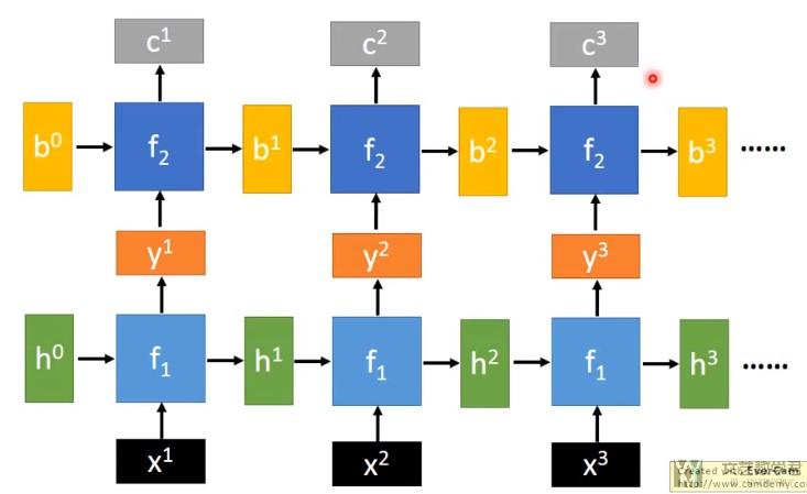
相当于每一层都有一个hidden state, 这里的h和b都是表示hidden state。当然,在具体写的时候,只需要修改num_layer的参数即可。(具体Pytorch中RNN的使用看下面讲Bidirectional RNN, 双向RNN)
Bidirectional RNN
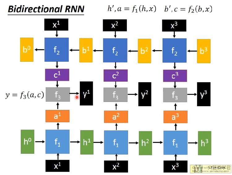
关于使用Bidirectional RNN(双向RNN)的好处为, 可以使得Network看的范围更加广了,因为network不仅从句首看到句末,也从句末看到句首;
关于Bidirectional RNN的结构如下所示,可以看到有上下两个方向的RNN, 一个是从x1向x3, 一个是x3向x1(看输入).
在PyTorch中,我们只需要设置bidirectional = True即可。如下所示。
- # ------------------------------
- # layer=1, bidirectional双向网络
- # -----------------------------
- N_INPUT = 4 # number of features in input
- N_OUTPUT = 2 #number of features in output
- N_BATCHSIZE = 3 # batchsize in input
- N_LAYERS = 1
- x_batch = torch.tensor([[[1,2,3,0],[4,5,6,1],[2,7,8,9]],[[1,2,3,0],[4,5,6,1],[2,7,8,9]],[[1,0,0,1],[1,1,0,0],[1,1,1,1]]]).float()
- # 初始化网络
- rnn = nn.RNN(input_size = N_INPUT, hidden_size = N_OUTPUT, num_layers = N_LAYERS, nonlinearity = 'relu', bias = False, bidirectional = True)
- # 初始化网络的系数
- rnn.weight_ih_l0.data = torch.ones(N_OUTPUT,N_INPUT).float()
- rnn.weight_hh_l0.data = 0.5*torch.ones(N_OUTPUT,N_OUTPUT)
- rnn.weight_ih_l0_reverse.data = 0.5*torch.ones(N_OUTPUT,N_INPUT)
- rnn.weight_hh_l0_reverse.data = 0.5*torch.ones(N_OUTPUT,N_OUTPUT)
- # 初始化memory
- initial_memory = torch.zeros(N_LAYERS*2, N_BATCHSIZE, N_OUTPUT)
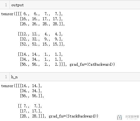
- output, h_n = rnn(x_batch,initial_memory)
我们简单使用上面的举一下例子,看一下最后结果的输出。
关于上面值得计算,可以参考下面得计算过程,其中weight得初始话在图中有,如果图片不清楚,可以直接看上面代码中得初始化得值。
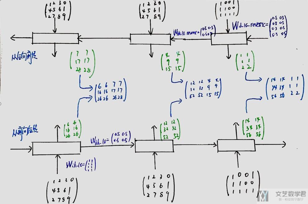
上面是关于简单得RNN的一些介绍,包括最基本的RNN的计算,layer>1的情况下的计算和双向RNN的计算。
RNNCell的简单记录
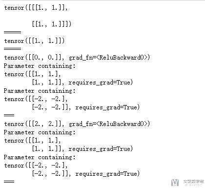
在Pytorch中,可以直接使用RNNCell,这个会比RNN更加自由一些。下面看一个简单的使用。
- rnn = nn.RNNCell(input_size=2, hidden_size=2, bias=False, nonlinearity='relu')
- # 初始化rnn的weight
- rnn.weight_ih.data = torch.ones(2,2)
- rnn.weight_hh.data = -2*torch.ones(2,2)
在使用RNNCell的时候,input需要自己来传入(可能讲的不怎么对, 我自己一般不用RNNCell)。
- # 其实就是把上一次的输出值, 作为输出输入下一次的网络
- # 可以看到输入一样的值, 但是输出是不一样的
- input = torch.ones(2, 1, 2)
- print(input)
- print('=====')
- hx = torch.ones(1, 2)
- print(hx)
- print('=====')
- output = []
- for i in range(2):
- hx = rnn(input[i], hx)
- print(hx)
- print(rnn.weight_ih) # input-hidden weights
- print(rnn.weight_hh) # hidden-hidden weights
- output.append(hx)
- print('===')
Simple RNN的问题
上面我们介绍了最简单的RNN,但是实际在使用的时候Simple RNN会有一些缺点,并且比较难被训练(这个之后讲BPTT的时候会讲到, 讲RNN的反向传播)
我们先举一个比较实际的例子
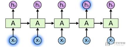
Sometimes, we only need to look at recent information to perform the present task. For example, consider a language model trying to predict the next word based on the previous ones. If we are trying to predict the last word in "the clouds are in the sky," we don't need any further context – it's pretty obvious the next word is going to be sky. In such cases, where the gap between the relevant information and the place that it's needed is small, RNNs can learn to use the past information.(有些时候,比如预测上下问,我们只需要关注前面的一个或几个单词,不会距离太远,如下图中我们认为h3是与x1有关的)
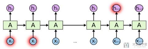
But there are also cases where we need more context. Consider trying to predict the last word in the text "I grew up in France… I speak fluent French." Recent information suggests that the next word is probably the name of a language, but if we want to narrow down which language, we need the context of France, from further back. It's entirely possible for the gap between the relevant information and the point where it is needed to become very large.(但有的时候,我们预测的词与前面有关联的词会相距比较远的距离。就像下图所示,h_t+1与x_1有关, 但是他们相隔很远)
对于这种情况,使用简单的RNN就是无法进行解决的(很难训练起来)。所以我们下面介绍一下LSTM和GRU,这两种都是为了解决RNN训练不起来,也就是出现梯度消失的问题.(梯度爆炸可以使用梯度截断来进行处理)
Long Short-term Memory (LSTM)-1997
这一部分会简单介绍一下LSTM的相关内容,主要说一下LSTM是如何进行具体的计算工作的。
LSTM的大致内容如下:
- LSTM也是只有短期记忆(short-term), 只不过会比Simple RNN长一些(通过gate来进行控制);
- LSTM有3*gate+1*input, 参数是普通的RNN的四倍;
- 通过操作3个gate, 使得memory不会被每次清除;
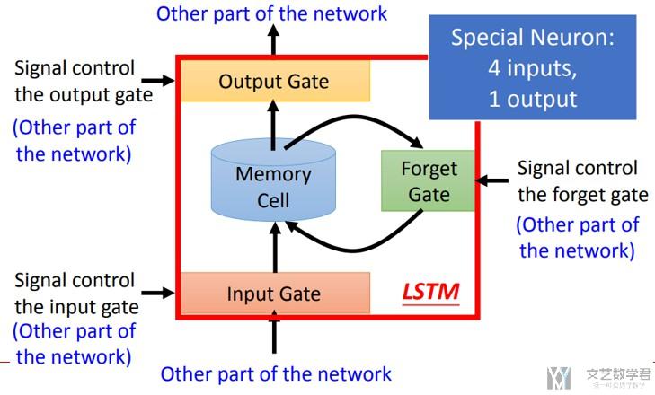
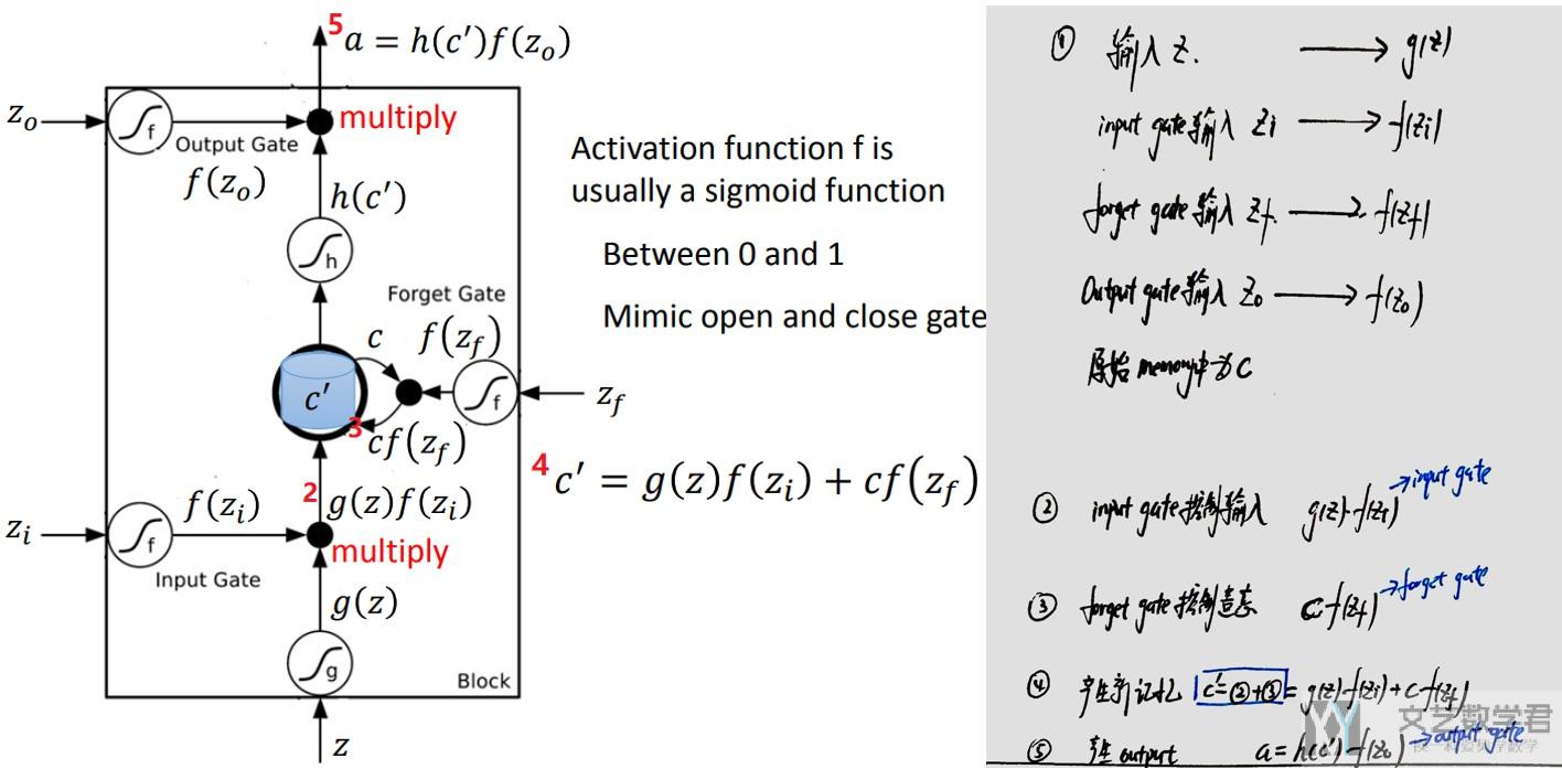
我们看一下LSTM的基本结构,他会有三个gate来控制input, forget和output,大致的示意图如下所示。
我们来看一下具体的计算的过程,下图中左边使用红色标出的序号与右边的计算的式子相互对应。可以看到,有四个参数z为输入, z_i控制input gate, z_f控制forget gate, z_o控制output gate.
对于整体的计算的步骤
- input gate控制input date的输入.
- forget gate控制是否遗忘cell state(之前的记忆)
- 接着产生新的记忆, 即进入input gate的值和经过forget gate的值(原来在memory中的值)
- 最后产生的值经过output gate
可以对照着下面的图看一下。左边是LSTM整个流程图,右边是计算的式子。
那么,控制三个gate的参数, z_i, z_f和z_f都是什么呢。下面简单解释一下。(下图可以点击查看大图)
我们可以理解为这三个系数, 是我们将输入x_t和上一次的hidden state拼接, 通过乘系数W得到的. 这里的系数是需要学习得到的。所以LSTM需要学习的系数的个数是Simple RNN的四倍(这里会有四个系数,分别对应下右图中的W_ii(input gate), W_if(forget gate), W_io(output gate)和W_ig)。
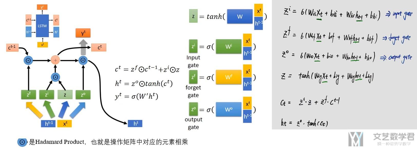
我们注意到,与Simple RNN比较, 在LSTM中, Cell State的值不会每次都被遗忘掉。
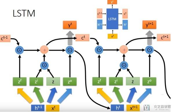
对于输入是sequence的时候,我们只需要接下去即可,如下图所示.
我们还需要注意到,Simple RNN就是一个特殊的LSTM,当把input gate和output gate全部设置为1,forget gate全部设置为0即可。
If you fix the input gate all 1's, the forget gate to all 0's (you always forget the previous memory) and the output gate to all 1's (you expose the whole memory) you almost get standard RNN.
为了更好的理解,我们举一个具体的算例。
LSTM具体算例
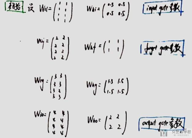
我们用Pytorch来算一下,我们通过使系数初始化成我们方便计算的数字。
- # -------------
- # LSTM, layer=1
- # -------------
- N_INPUT = 4 # number of features in input
- N_OUTPUT = 2 #number of features in output
- N_BATCHSIZE = 3 # batchsize in input
- N_LAYERS = 1
- x_batch = torch.tensor([[[1,2,3,0],[4,5,6,1],[2,7,8,9]],[[1,0,0,1],[1,1,0,0],[1,1,1,1]]]).float()
- # 初始化网络
- rnn = nn.LSTM(input_size = N_INPUT, hidden_size = N_OUTPUT, num_layers = N_LAYERS, bias = False, bidirectional = False)
- # 初始化网络的系数
- # 参数出现的顺序, W_ii|W_if|W_ig|W_io
- parameters = torch.ones(4*N_OUTPUT,N_INPUT)
- parameters[2:4] = 2*parameters[2:4]
- parameters[4:6] = 3*parameters[4:6]
- parameters[6:8] = 4*parameters[6:8]
- rnn.weight_ih_l0.data = parameters
- parameters = 0.5*torch.ones(4*N_OUTPUT,N_OUTPUT)
- parameters[2:4] = 2*parameters[2:4]
- parameters[4:6] = 3*parameters[4:6]
- parameters[6:8] = 4*parameters[6:8]
- rnn.weight_hh_l0.data = parameters
- # 初始化memory
- h0 = torch.zeros(N_LAYERS, N_BATCHSIZE, N_OUTPUT)
- c0 = torch.zeros(N_LAYERS, N_BATCHSIZE, N_OUTPUT)
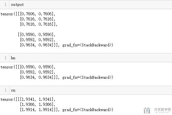
- output, (hn, cn) = rnn(x_batch,(c0,h0))
需要注意的是,LSTM是有两个hidden state(可以这么称呼),传入的时候也是需要有c_n(这个更像是memory)和h_n(h_n是和这个的output是相同的,可以看下面LSTM的输出)。
上面的网络等价与下图右边所示(可以打开新标签查看大图)。
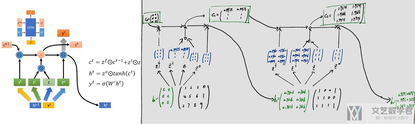
我们详细看一下第二段的计算,其实主要是利用上面讲的LSTM的计算公式,在这里我就是为了熟悉一下,最后和Pytorch计算的结果比较一下。
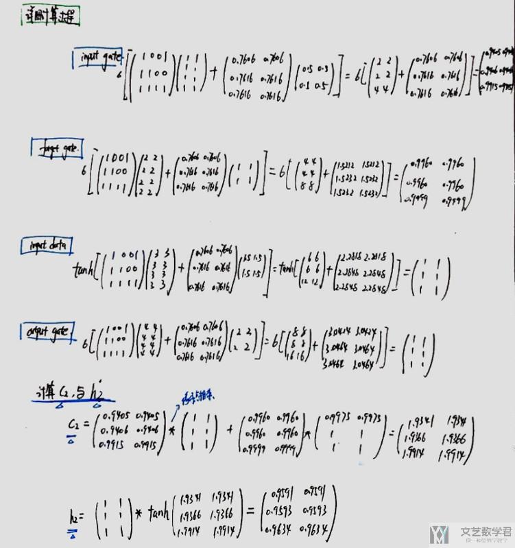
我们和Pytorch计算的结果比较一下,验证一下正确性.
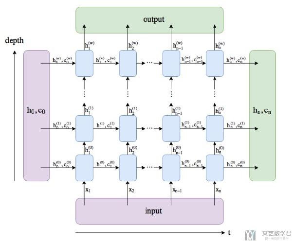
LSTM can be deep
同样,LSTM也是可以多层网络进行叠加的。我们具体看下面的这个图片。图片来源 : Clarification regarding the return of nn.GRU
Gated Recurrent Unit (GRU)-2014
关于GRU的相关内容,可以查看链接 : 人人都能看懂的GRU,这里有一些介绍。
GRU与LSTM相比,只有两个gate。GRU的总体计算流程如下所示:
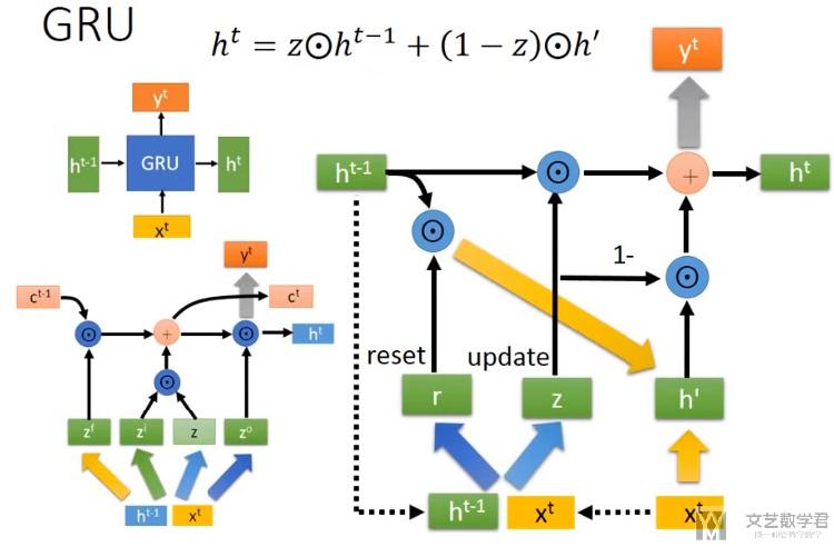
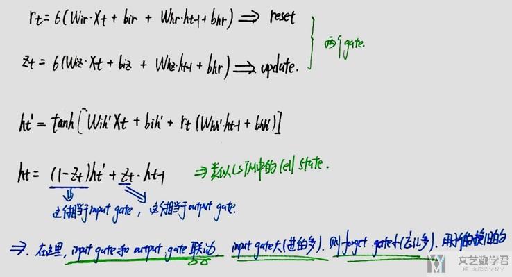
结合上图,我们看一下计算的过程:
- 上面的R_t表示reset gate,Z_t表示update gate
- The reset gate determines how to combine the new input with the previous memory.(其中reset gate的作用是来决定我们如何结合新的input和之前的memory)
- The update gate defines how much of the previous memory to keep around.(update的作用是我们如何结合之前的memory和现在的memory)
- If we set the reset to all 1's and update gate to all 0's we again arrive at our plain RNN model.(GRU与普通RNN的关系)
- 这里(1-z)相当于input gate
- Z相当于是forget gate(图上写错了, 不是output gate,应该是forget gate)
- 在这里input gate和forget gate是联动的, 若input gate大, 即输入的多, 那么forget gate小, 忘记的多.
关于GRU的性能
- GRU比LSTM少1/3的参数;
- 但是, GRU几乎拥有与LSTM相同的效果;
GRU简单实验
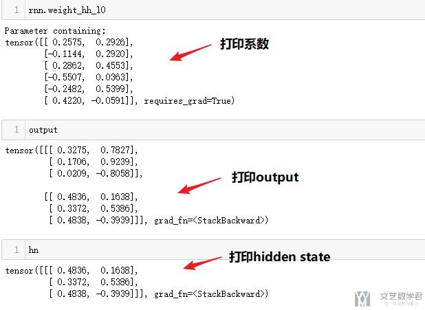
下面是在Pytorch中简单使用一下GRU的实验。简单看一下是如何使用的。
- # ------------------------------
- # GRU, layer=1
- # -----------------------------
- N_INPUT = 4 # number of features in input
- N_OUTPUT = 2 #number of features in output
- N_BATCHSIZE = 3 # batchsize in input
- N_LAYERS = 1
- x_batch = torch.tensor([[[1,2,3,0],[4,5,6,1],[2,7,8,9]],[[1,0,0,1],[1,1,0,0],[1,1,1,1]]]).float()
- # 初始化网络
- rnn = nn.GRU(input_size = N_INPUT, hidden_size = N_OUTPUT, num_layers = N_LAYERS, bias = False, bidirectional = False)
- # 初始化memory
- h0 = torch.zeros(N_LAYERS, N_BATCHSIZE, N_OUTPUT)
- output, hn = rnn(x_batch,h0)
结语

- 微信公众号
- 关注微信公众号
-

- QQ群
- 我们的QQ群号
-


评论