TensorFlow,Keras,PyTorch框架了解--实现线性回归

王茂南

2820
文章

75
评论

2018年7月15日23:25:18

评论2 5078字阅读16分55秒

摘要这一篇文章会介绍常用的三个深度学习的框架，TensorFlow、Keras和PyTorch。我会通过一个线性回归的例子来讲这三个框架的使用，把使用顺一遍。把三个框架放在一起，也是为了方便比较，和之后使用起来方便查找整体的流程。

文章目录(Table of Contents)

前言

这一篇会使用TensorFlow,Keras和PyTorch三种框架实现线性回归，也是作为简单了解一下这三种最常用的深度学习框架的使用。做这个线性回归，既可以顺一遍整个框架的流程，也不会太麻烦。

这三个框架，我个人使用起来觉得Keras是会方便一些(Keras底层是TensorFlow)，只不过又做了一次封装。PyTorch使用起来也不是很麻烦。怎么说呢，多用几次，多看看文档，多了解一下框架设计的时候的想法。

之后的话会实现一些经典的神经网络。

三种框架实现线性回归

首先我们先准备一下数据集：

数据准备

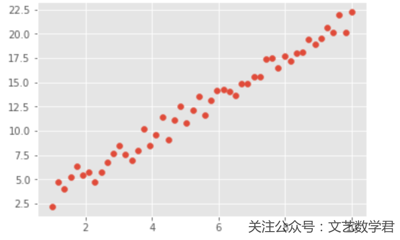
我们首先准备好需要回归的数据，并用图形显示出来：

import numpy as np
from matplotlib import pyplot as plt
%matplotlib inline
np.random.seed(7)
x = np.linspace(1, 10, 50)
y = 2 * x + 3 * np.random.rand(50)
plt.style.use("ggplot") # 使用美观的样式
plt.scatter(x, y)

下面我们依次按照TensorFlow，Keras和PyTorch这三个框架的顺序进行回归。

TensorFlow

TensorFlow文档
https://www.tensorflow.org/api_docs/python/

import tensorflow as tf
import os
# --------
# 初始化变量
# --------
X = x.reshape(-1,1)
Y = y.reshape(-1,1)
# 定义占位量,之后为了分批训练
x_batch = tf.placeholder(tf.float32, [None, 1])
y_batch = tf.placeholder(tf.float32, [None, 1])
# 需要预测的数据
X_pre = np.linspace(0, 11, 1000).reshape(-1,1)
# ---------
# 定义网络层
# ---------
dense_1 = tf.layers.dense(inputs=x_batch, units=1, activation=None)
# ---------
# 定义损失函数和优化器
# ---------
loss = tf.losses.mean_squared_error(labels=dense_1,predictions=y_batch)
# 优化器
learning_rate = 0.01
optimizer = tf.train.GradientDescentOptimizer(learning_rate = learning_rate)
training_op = optimizer.minimize(loss)
# -------
# 训练模型
# -------
batch_size = 25 # 定义batch_size
init = tf.global_variables_initializer() # 之后可以对所有节点初始化
n_epochs = 10
loss_list = [] # 存储训练的误差
with tf.Session() as sess:
sess.run(init)
for epochs in range(n_epochs):
train_batch = zip(range(0, len(x), batch_size), range(batch_size, len(x) + 1, batch_size))
i = 0
for start, end in train_batch:
X_batch = X[start:end] # 获得X的小批量训练数据
Y_batch = Y[start:end] # 获得Y的小批量训练数据
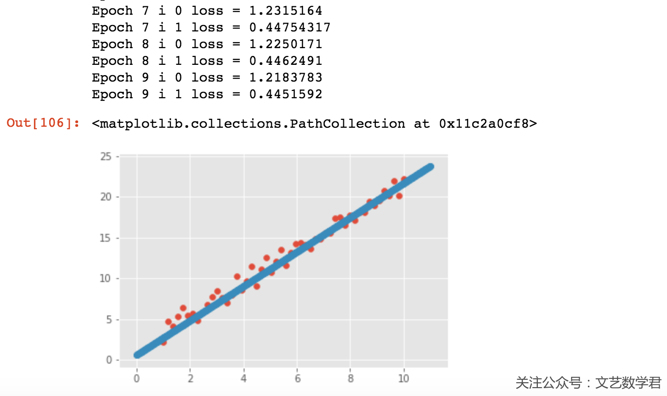
loss_epoch = sess.run(loss, feed_dict={x_batch: X_batch, y_batch: Y_batch}) # 计算误差
print("Epoch", epochs, 'i', i, "loss =", loss_epoch)
loss_list.append(loss_epoch)
sess.run(training_op, feed_dict={x_batch: X_batch, y_batch: Y_batch}) # 进行反向传播
i = i + 1
result = sess.run(dense_1, feed_dict={x_batch : X_pre})
# ----------
# 绘制预测图像
# ----------
plt.style.use("ggplot") # 使用美观的样式
plt.scatter(x, y)
plt.scatter(X_pre,result)

上面就是使用TensorFlow进行回归的整个流程，虽然只有50个数据，但是作为样例还是使用了batch进行训练。

我们看一下部分输出，训练10次，每次传入25个数据进行训练，从图像上看直线拟合效果还是很好的：

Keras

Keras文档
https://keras-cn.readthedocs.io/en/latest/

from keras.models import Sequential
from keras.layers import Dense
# --------
# 初始化数据
# --------
X = x # 就是numpy的类型
Y = y
# ------
# 模型构建
# ------
model = Sequential() # 声明序贯模型
# 这里input_dim为输入向量的维度,units为输出的维度
model.add(Dense(input_dim=1, units=1))
# -------
# 定义模型的损失函数与优化器
# -------
model.compile(loss='mean_squared_error', optimizer='sgd')
# -------
# 模型训练
# -------
model.fit(X, Y, epochs=10, batch_size=32)
# ----------
# 画出拟合图像
# ----------
weight = model.get_weights()[0] # 权重
bias = model.get_weights()[1] # 偏置项
plt.style.use("ggplot") # 使用美观的样式
plt.scatter(x, y)
x_plot = np.linspace(1, 10, 500)
print('weight : ', weight, 'bias : ', bias)
plt.plot(x_plot, (weight*x_plot+bias).flatten(), c='black') # 这里要转为numpy才能绘制

可以看到Keras的代码会比上面使用TensorFlow少一些，同时使用Keras来设置批训练等是很方便的。我们这里训练了10次，可以看一下最后部分输出的结果和拟合的图像：

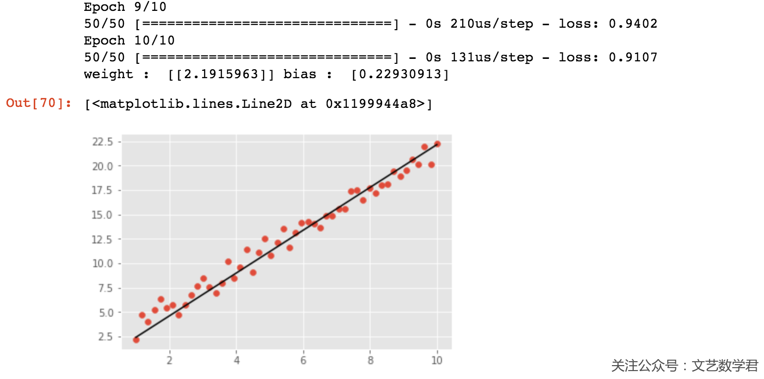
同样可以看到直线的拟合效果还是很不错的。

PyTorch

PyTorch文档
https://pytorch.org/docs/stable/index.html

import torch as t
import torch.nn as nn
from torch.nn.functional import sigmoid
from torch import optim
from torch.autograd import Variable
import torch.utils.data as Data
# -------
# 定义网络
# -------
class LinearRegressionModel(nn.Module):
def __init__(self):
super(LinearRegressionModel, self).__init__() # 等价于 nn.Module.__init__(self)
self.linear1 = nn.Linear(1, 1)
def forward(self, x):
out = self.linear1(x)
return out
# ------
# 定义损失函数和优化器
# ------
model = LinearRegressionModel() # 实例化模型
loss_fn = nn.MSELoss(size_average=True) # 定义损失函数,这里True表示会求平均
optimiser = optim.SGD(params=model.parameters(), lr=0.01) # 定义优化器
# ------
# 定义变量
# ------
X = t.Tensor(x).reshape(-1,1) # 输入 x 张量
# X = Variable(x.reshape(len(x),1)) # 也可以通过这种方式进行shape的转换
Y = t.Tensor(y).reshape(-1,1) # 输入 y 张量
# 使用batch训练
torch_dataset = Data.TensorDataset(X, Y) # 合并训练数据和目标数据
MINIBATCH_SIZE = 25
loader = Data.DataLoader(
dataset=torch_dataset,
batch_size=MINIBATCH_SIZE,
shuffle=True,
num_workers=2 # set multi-work num read data
)
# ------
# 进行训练
# ------
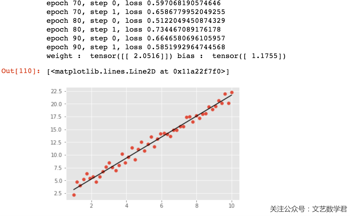
for epoch in range(100):
for step, (batch_x, batch_y) in enumerate(loader):
optimiser.zero_grad() # 梯度清零
out = model(batch_x) # 前向传播
loss = loss_fn(out, batch_y) # 计算损失
loss.backward() # 反向传播
optimiser.step() # 随机梯度下降
if epoch % 10 == 0:
print('epoch {}, step {}, loss {}'.format(epoch, step, loss.item()))
# ----------
# 画出拟合图像
# ----------
weight = model.state_dict()['linear1.weight'] # 权重
bias = model.state_dict()['linear1.bias'] # 偏置项
plt.style.use("ggplot") # 使用美观的样式
plt.scatter(x, y)
x_plot = np.linspace(1, 10, 500)
# 注意下面的 tensor转numpy
print('weight : ', weight, 'bias : ', bias)
plt.plot(x_plot, (weight.numpy()*x_plot+bias.numpy()).flatten(), c='black') # 这里要转为numpy才能绘制