文章目录(Table of Contents)
简介
有的时候,我们想要了解卷积层的某个filter是在检测什么特征,于是想要对其进行一些可视化的解释。这里会讲的一种方法,主要的思想是找一张图片,使得某个layer的filter的激活值最大,这张图片就是能被这个filter所检测的对象。
特别说明:这里的初始对象,一般会有两种方式,如下:
- 输入一堆图片,找出其中一张,使得某个神经元激活最大
- 随机给一张图片,通过梯度下降,修改这张图片的像素,是某个神经元的激活最大
接下来会讲的是第二种方法。
关于filter的激活值
关于filter的激活值,我们可以使用下面的定义,其实相当于给定了一个loss函数,可以进行梯度下降,进行反复迭代。
- 如现在filter的输出为11*11的一个矩阵(经过一个卷积层的输出)
- 下图a_ij_k表示第k个filter的第i行j列;
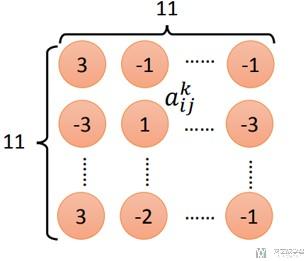
- 对输出值进行求和(这里的定义可以根据需要进行改变);
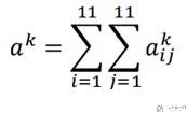
- 最终的目标是使得a_k最大;
- 最终,使用梯度下降法进行求解;
最后,十分建议阅读下面的参考链接,原文给出了更加详细的解释。我也是模仿的他的进行的实验。
参考链接:How to visualize convolutional features in 40 lines of code
一些其他的CNN可视化的链接
- CS231n Convolutional Neural Networks for Visual Recognition
- Convolutional Neural Network Visualizations--Pytorch
方法简单介绍
其实根据上面的如何计算filter的激活值,我们就可以大致知道步骤是什么了。这里简单叙述一下,因为在实际的使用过程中,会有一些小的tricks,会关系到最后图像生成的效果的好坏。
- 初始化一张图片, 56*56
- 使用预训练好的VGG16网络,固定网络参数;
- 若想可视化第40层layer的第k个filter的conv, 我们设置loss函数为 (-1*神经元激活值);
- 梯度下降, 对初始图片进行更新;
- 对得到的图片*1.2, 得到新的图片,重复上面的步骤;
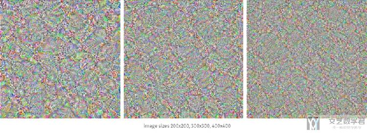
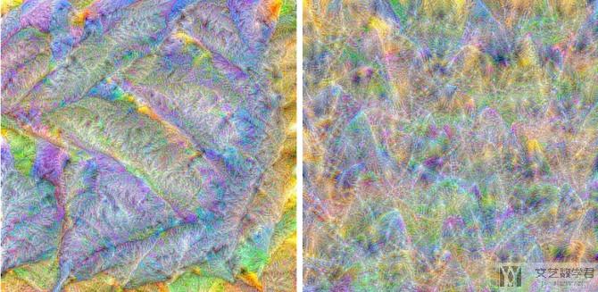
其中第五步比较关键,我们可以看到初始化的图片不是很大,只有56*56. 这是因为原文作者在实际做的时候发现,若初始图片较大,得到的特征的频率会较高,即没有现在这么好的显示效果。
就像下图所展示,图像的size小的时候,pattern更加明显。所以在实际的操作中,会有第五步,就是希望初始化的图片从较小的开始,逐渐变大,使得最后的特征不会频率很高,导致无法看清。
下面我们先看一下结果的分析,关于具体的实现会在最后一部分进行说明。
简单分析
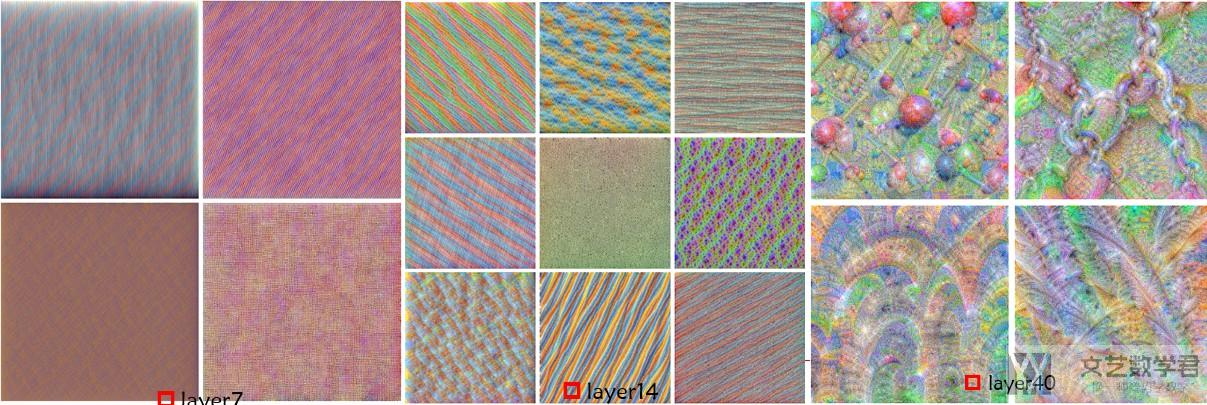
随着卷积层的加深, pattern在变得复杂
下面从左到右,分别是layer7, layer14和layer40画出的效果图, 随着layer的增加,卷积层所能检测的pattern在变得复杂。
验证猜想
比如对于layer 40, filter 64,绘制出的结果如下图所示。我们可以看出包含羽毛,鸟的脚部与头部,我们想要验证一下这个filter是否在输入鸟的图片时,可以得到比较大的激活值(这是验证的方法)。
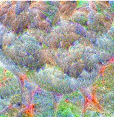
于是,我们准备一张鸟的图片,输入网络,图片如下所示:
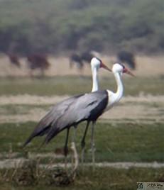
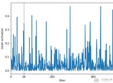
于是我们可以得到layer40上,每一个filter被激活的程度。可以看到在64个filter上激活值还是很大的。同时,在其他的几层上,也有较大的激活值,我们把那些位置的filter对于的图片均画出.
其中,有些是具有可解释性的,我们仍能看到一些鸟的特征,如下所示:
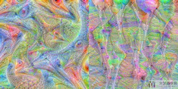
但是,有些filter不具有可解释性,作者在原文是这样解释的,即可能这些pattern与背景有关,或是一些网络需要一起用来判断鸟类。
Regarding the bottom row, however, I have no clue. Maybe those patterns are associated with the background of the image or simply represent something the network needs for detecting birds that I don’t understand. I suppose this will remain part of the black box for now…
代码实现
导入相应的库
- import torch
- from torch.autograd import Variable
- from PIL import Image,ImageOps
- import torchvision.transforms as transforms
- import torchvision.models as models
- import numpy as np
- import cv2
- from cv2 import resize
- from matplotlib import pyplot as plt
- %matplotlib inline
设置device变量,用来控制是否使用cuda
- device = torch.device('cuda' if torch.cuda.is_available() else 'cpu')
初始化图片
我们需要注意的是,这里我们要更新的是图片,网络的weight是不变的。
- # 生成随机的图片
- sz = 56
- img = np.uint8(np.random.uniform(150, 180, (3, sz, sz)))/255
- # img[None]可以增加一个维度
- img = torch.from_numpy(img[None]).float().to(device)
- img.shape
- # torch.Size([1, 3, 56, 56])
导入预训练好的网络
在这里使用带有batchnorm的VGG16。
- model_vgg16 = models.vgg16_bn(pretrained=True).features.to(device).eval()
使用hook类
在pytorch中,我们需要使用hook来得到网络中间层的输出。在这里我们先写好类,之后可以方便进行使用。方便得到某个layer的所有filter的输出。
- class SaveFeatures():
- """注册hook和移除hook
- """
- def __init__(self, module):
- self.hook = module.register_forward_hook(self.hook_fn)
- def hook_fn(self, module, input, output):
- # self.features = output.clone().detach().requires_grad_(True)
- self.features = output.clone()
- def close(self):
- self.hook.remove()
接着,我们将其注册到layer40.
- layer = 40
- activations = SaveFeatures(list(model_vgg16.children())[layer])
进行反向传播
我们首先先定义超参数,其中upscaling_steps就是上面讲方法介绍的第五步,逐步放大图像的次数,这里选择了13次。upscaling_factor就是每次放大的倍数。blur是每次放大后会有一个模糊的处理,也是为了让最后的效果变得更好。
- # 超参数
- lr = 0.1 # 学习率
- opt_steps = 25 # 迭代次数
- filters = 265 # 第265个filter,使其最大
- upscaling_steps = 13 # 图像放大次数
- blur=3
- upscaling_factor=1.2 # 把图像变粗
接着我们还需要设置一下均值和方差,这是由于VGG16网络会对输出进行normalization,所以我们需要自己对输入进行标准化。
- # 定义处理时的均值与方差
- cnn_normalization_mean = torch.tensor([0.485, 0.456, 0.406]).view(-1, 1, 1).to(device)
- cnn_normalization_std = torch.tensor([0.229, 0.224, 0.225]).view(-1, 1, 1).to(device)
最后就是进行梯度下降即可。注意一定要移除hook在最后。
- for epoch in range(upscaling_steps): # scale the image up upscaling_steps times
- # --------------------------------------------------------------------------------
- # 因为原始的VGG网络对图片做了normalization, 所以这里对输入图片也要做normalization
- # --------------------------------------------------------------------------------
- img = (img - cnn_normalization_mean) / cnn_normalization_std
- img=1
- img=0
- print('Imgshape1 : ',img.shape)
- img_var = Variable(img, requires_grad=True) # convert image to Variable that requires grad
- # ----------
- # 定义优化器
- # ----------
- optimizer = torch.optim.Adam([img_var], lr=lr, weight_decay=1e-6)
- for n in range(opt_steps): # optimize pixel values for opt_steps times
- optimizer.zero_grad()
- model_vgg16(img_var) # 正向传播
- loss = -activations.features[0, filters].mean() # loss相当于最大该层的激活的值
- loss.backward()
- optimizer.step()
- # ------------
- # 图像进行还原
- # ------------
- print('Loss:',loss.cpu().detach().numpy())
- img = img_var * cnn_normalization_std + cnn_normalization_mean # 这个使用img_var变换img
- img=1
- img=0
- img = img.data.cpu().numpy()[0].transpose(1,2,0)
- sz = int(upscaling_factor * sz) # calculate new image size
- img = cv2.resize(img, (sz, sz), interpolation = cv2.INTER_CUBIC) # scale image up
- if blur is not None: img = cv2.blur(img,(blur,blur)) # blur image to reduce high frequency patterns
- print('Imgshape2 : ',img.shape)
- img = torch.from_numpy(img.transpose(2,0,1)[None]).to(device)
- print('Imgshape3 : ',img.shape)
- print(str(epoch),',Finished')
- print('=======')
- activations.close() # 移除hook
最后将图像进行保存即可。
- # 保存图片
- image = img.cpu().clone()
- image = image.squeeze(0)
- unloader = transforms.ToPILImage()
- image = unloader(image)
- image = cv2.cvtColor(np.asarray(image),cv2.COLOR_RGB2BGR)
- cv2.imwrite('res1.jpg',image)
- torch.cuda.empty_cache()
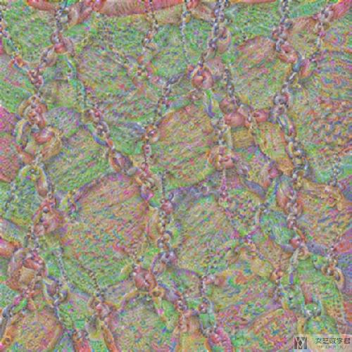
看一下最终的效果。可以看到图中包含链条的形状,我们接下来进行验证结果。
验证结果
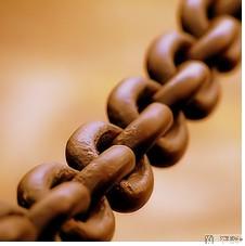
首先导入验证的图片。
- size = (224, 224)
- picture = Image.open("./Broad_chain_closeup.jpg")
- # picture = Image.open("./Wattledcranethumb.jpg")
- picture = ImageOps.fit(picture, size, Image.ANTIALIAS)
- picture
- # 转换为tensor
- loader = transforms.ToTensor()
- picture = loader(picture).to(device)
- # 将图片做标准化, 转换为vgg网络的输入
- cnn_normalization_mean = torch.tensor([0.485, 0.456, 0.406]).view(-1, 1, 1).to(device)
- cnn_normalization_std = torch.tensor([0.229, 0.224, 0.225]).view(-1, 1, 1).to(device)
- # 减均值. 除方差
- picture = (picture - cnn_normalization_mean) / cnn_normalization_std
- # 查看转换之后的效果
- # unload = transforms.ToPILImage()
- # unload(picture.cpu())
接着,使用这张图片在网络中进行传播,并得到layer42的输出。这里使用layer42是因为layer42是经过ReLU之后,可以均为正数。写成layer40也是可以的。
- # 定义网络
- model_vgg16 = models.vgg16_bn(pretrained=True).features.to(device).eval()
- # 对网络进行hook,hook住指定层的output的值
- layer = 42 # 这里是ReLU之后, 经过激活之后也应该较大
- filters = 265
- activations = SaveFeatures(list(model_vgg16.children())[layer])
- # 网络前向传播
- with torch.no_grad():
- picture_var = Variable(picture[None])
- model_vgg16(picture_var)
- activations.close() # 移除hook
最后绘制出所有filter的均值即可。
- # 画出每个filter的平均值
- mean_act = [activations.features[0,i].mean().item() for i in range(512)] # 计算平均值
- plt.figure(figsize=(7,5))
- act = plt.plot(mean_act,linewidth=2.) # 画出折线图
- extraticks=[filters] # 增加的一个坐标
- ax = act[0].axes
- ax.set_xlim(0,500)
- plt.axvline(x=filters, color='grey', linestyle='--') # 绘制虚线
- ax.set_xlabel("feature map")
- ax.set_ylabel("mean activation")
- ax.set_xticks([0,200,400] + extraticks)
- plt.show()
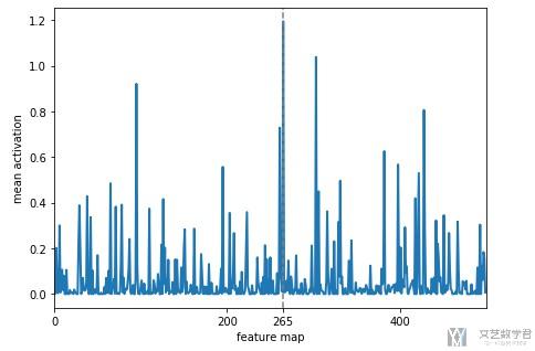
可以看到filter=265时候,激活的值是比较大的。
结语
以上就是整个详细的流程。详细的代码可以参考下面的链接。我已上传了完整的代码。
关于feature map的绘制,在Pytorch forum上也是有提及的,地址如下,Visualize feature map
- 微信公众号
- 关注微信公众号
-

- QQ群
- 我们的QQ群号
-


评论