文章目录(Table of Contents)
简介
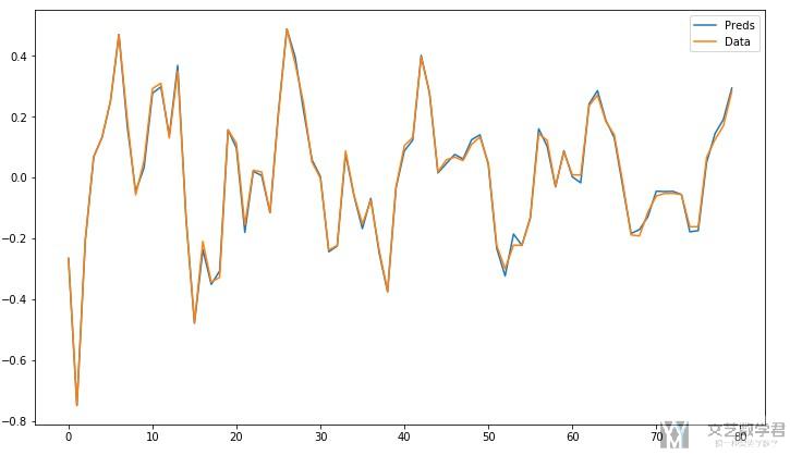
这一篇文章,会完成使用RNN, 更具体的说是使用GRU来实现时间序列的分析, 用来做预测. 最终的效果如下, 后面会有每一步的具体步骤。
主要参考的文章为下面两篇文章 :
- LSTMs for Time Series in PyTorch : 数据的来源(生成AR(5) data)
- Time Series in Python — Part 3: Forecasting taxi trips with LSTMs : 整体的思想(参考了一下这篇文章网络的书写)
数据输入
在处理时间序列数据的时候,对于输入我们有两种处理的办法。我们会将数据分为chunk。
如图一, 比如我们使用前6天预测第七天, 再使用前七天预测第八天, 以此类推.
如图二, 比如我们使用0-6天预测第七天, 使用1-7天预测第八天, 以此类推.
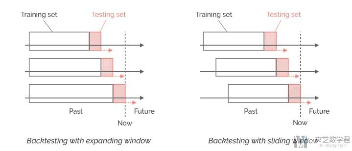
在我们这篇文章,我们会采取使用图2的形式. 我们会以7天作为一个阶段, 使用七天的数据预测第八天.
In our case study, I will use samples consisting of 7-days sliding windows with step size equal to 1, used to predict the next value (1-step ahead forecast).
下面我们看一下具体的实现。这里一段内容参考自上面的链接二。
具体的实现
导入所需要的库
- import torch
- import torch.nn as nn
- import torch.optim as optim
- import numpy as np
- from sklearn.model_selection import train_test_split
- import matplotlib.pyplot as plt
Generating Autoregressive data for experiments(生成所需要的数据)
这里的代码来自上面的链接一, 我在代码注释中也写了来源, 这个数据我没仔细看, 后面就是直接使用了。
- # 代码来源 : http://www.jessicayung.com/generating-autoregressive-data-for-experiments/
- # 代码来源 : https://github.com/jessicayung/blog-code-snippets
- class TimeSeriesData:
- def __init__(self, num_datapoints, test_size=0.2, max_t=20, num_prev=1,
- noise_var=1):
- """
- Template class for generating time series data.
- :param test_size: in (0,1), data to be used in test set as a fraction of all data generated.
- """
- self.num_datapoints = num_datapoints
- self.test_size = test_size
- self.num_prev = num_prev
- self.max_t = max_t
- self.data = None
- self.noise_var = noise_var
- self.y = np.zeros(num_datapoints + num_prev*4) # TODO: check this
- self.bayes_preds = np.copycopy(self.y)
- # Generate data and reshape data
- self.create_data()
- # Split into training and test sets
- self.train_test_split()
- def create_data(self):
- self.generate_data()
- self.reshape_data()
- def generate_data(self):
- """Generates data in self.y, may take as implicit input timesteps self.t.
- May also generate Bayes predictions."""
- raise NotImplementedError("Generate data method not implemented.")
- def reshape_data(self):
- self.x = np.reshape([self.y[i:i + self.num_prev] for i in range(
- self.num_datapoints)], (-1, self.num_prev))
- self.y = np.copycopy(self.y[self.num_prev:])
- self.bayes_preds = np.copycopy(self.bayes_preds[self.num_prev:])
- def train_test_split(self):
- test_size = int(len(self.y) * self.test_size)
- self.data = [self.X_train, self.X_test, self.y_train,
- self.y_test] = \
- self.x[:-test_size], self.x[-test_size:], \
- self.y[:-test_size], self.y[-test_size:]
- self.bayes_preds = [self.bayes_train_preds, self.bayes_test_preds] = self.bayes_preds[:-test_size], self.bayes_preds[-test_size:]
- def return_data(self):
- return self.data
- def return_train_test(self):
- return self.X_train, self.y_train, self.X_test, self.y_test
- class ARData(TimeSeriesData):
- """Class to generate autoregressive data."""
- def __init__(self, *args, coeffs=None, **kwargs):
- self.given_coeffs = coeffs
- super(ARData, self).__init__(*args, **kwargs)
- if coeffs is not None:
- self.num_prev = len(coeffs) - 1
- def generate_data(self):
- self.generate_coefficients()
- self.generate_initial_points()
- # + 3*self.num_prev because we want to cut first (3*self.num_prev) datapoints later
- # so dist is more stationary (else initial num_prev datapoints will stand out as diff dist)
- for i in range(self.num_datapoints+3*self.num_prev):
- # Generate y value if there was no noise
- # (equivalent to Bayes predictions: predictions from oracle that knows true parameters (coefficients))
- self.bayes_preds[i + self.num_prev] = np.dot(self.y[i:self.num_prev+i][::-1], self.coeffs)
- # Add noise
- self.y[i + self.num_prev] = self.bayes_preds[i + self.num_prev] + self.noise()
- # Cut first 20 points so dist is roughly stationary
- self.bayes_preds = self.bayes_preds[3*self.num_prev:]
- self.y = self.y[3*self.num_prev:]
- def generate_coefficients(self):
- if self.given_coeffs is not None:
- self.coeffs = self.given_coeffs
- else:
- filter_stable = False
- # Keep generating coefficients until we come across a set of coefficients
- # that correspond to stable poles
- while not filter_stable:
- true_theta = np.random.random(self.num_prev) - 0.5
- coefficients = np.append(1, -true_theta)
- # check if magnitude of all poles is less than one
- if np.max(np.abs(np.roots(coefficients))) < 1:
- filter_stable = True
- self.coeffs = true_theta
- def generate_initial_points(self):
- # Initial datapoints distributed as N(0,1)
- self.y[:self.num_prev] = np.random.randn(self.num_prev)
- def noise(self):
- # Noise distributed as N(0, self.noise_var)
- return self.noise_var * np.random.randn()
- # A set of coefficients that are stable (to produce replicable plots, experiments)
- fixed_ar_coefficients = {2: [ 0.46152873, -0.29890739],
- 5: [ 0.02519834, -0.24396899, 0.2785921, 0.14682383, 0.39390468],
- 10: [-0.10958935, -0.34564819, 0.3682048, 0.3134046, -0.21553732, 0.34613629,
- 0.41916508, 0.0165352, 0.14163503, -0.38844378],
- 20: [ 0.1937815, 0.01201026, 0.00464018, -0.21887467, -0.20113385, -0.02322278,
- 0.34285319, -0.21069086, 0.06604683, -0.22377364, 0.11714593, -0.07122126,
- -0.16346554, 0.03174824, 0.308584, 0.06881604, 0.24840789, -0.32735569,
- 0.21939492, 0.3996207 ]}
使用上面的代码生成我们需要的数据, 这样我们就有了训练和测试的时候需要的数据了。
- #####################
- # Generate data
- #####################
- num_datapoints = 100
- test_size = 0.2
- input_size = 20
- noise_var = 0
- data = ARData(num_datapoints, num_prev=input_size, test_size=test_size, noise_var=noise_var, coeffs=fixed_ar_coefficients[input_size])
- # --------------------
- # Device configuration
- # --------------------
- device = torch.device('cuda' if torch.cuda.is_available() else 'cpu')
- # data for train and test
- X_train = torch.from_numpy(data.X_train).float().to(device)
- X_test = torch.from_numpy(data.X_test).float().to(device)
- y_train = torch.from_numpy(data.y_train).float().to(device)
- y_test = torch.from_numpy(data.y_test).float().to(device)
定义生成器(用于逐次生成训练的数据)
根据上面我们介绍的,我们需要每七天的数据作为一组,进入模型进行训练. 如我们需要逐次返回 :
- 3/1-3/7的数据为训练集, 3/8为需要预测的;
- 3/2-3/8的数据为训练集, 3/9为需要预测的
- 3/3-3/9的数据为训练集, 3/10为需要预测的
- ...
于是我们使用yield, 最后可以返回一个生成器.
- # 使用slide window, window size=7
- # 即返回 data=1-7 label=8; data=2-8 label=9
- def create_dataset(X_data, y_data, look_back=1):
- length = X_data.size(0)
- for i in range(0,length-look_back):
- result = (X_data[i:(i+look_back),:],y_data[i+look_back])
- yield result
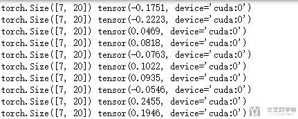
简单测试一下,就是可以逐次返回训练的样本和target.
- test_data = create_dataset(X_train,y_train, look_back=7)
- for (i,j) in test_data:
- print(i.shape,j)
定义网络
接下来我们定义预测所需要的网络结构。
- class TimeSeries(nn.Module):
- def __init__(self, input_dim, hidden_dim, batch_size, output_dim=1, num_layers=2):
- super(TimeSeries,self).__init__()
- self.input_dim = input_dim # 输入的特征的个数
- self.hidden_dim = hidden_dim
- self.batch_size = batch_size
- self.num_layers = num_layers
- self.output_dim = output_dim
- # Defeine the GRU layer
- self.gru = nn.GRU(self.input_dim, self.hidden_dim, self.num_layers, dropout=0.1)
- # Define the output layer
- self.fc = nn.Linear(self.hidden_dim, self.output_dim)
- def init_hidden(self):
- # initialise hidden state
- return (torch.zeros(self.num_layers, self.batch_size, self.hidden_dim).to(device))
- # return (torch.zeros(self.num_layers, self.batch_size, self.hidden_dim))
- def forward(self,x):
- self.batch_size = x.size(1)
- self.hidden = self.init_hidden() # 初始化hidden state
- gru_out, self.hidden = self.gru(x, self.hidden)
- y_pred = self.fc(gru_out[-1])
- return y_pred
简单测试一下网络的编写是否是正确的。
- # 模型的测试
- input_data = torch.from_numpy(np.random.randn(7,1,20)).float().to(device)
- model = TimeSeries(input_dim=20, hidden_dim=20, batch_size=1, output_dim=1, num_layers=2).to(device)
- model(input_data)
- """
- tensor([[-0.0021]], device='cuda:0', grad_fn=<AddmmBackward>)
- """
模型的训练
准备好模型和数据之后,我们就可以开始训练了。训练的代码如下所示:
- # 模型的初始化
- model = TimeSeries(input_dim=20, hidden_dim=28, batch_size=1, output_dim=1, num_layers=3).to(device)
- # 定义损失函数和优化器
- criterion = nn.MSELoss()
- optimizer = optim.Adam(model.parameters(),lr=0.001)
- # 模型的训练
- pre_output = y_train.clone()
- num_epochs = 1000
- hist = np.zeros(num_epochs) # 用来记录每一个epoch的误差
- for t in range(num_epochs):
- test_data = create_dataset(X_train,y_train, look_back=7) # 这个要每次刷新
- loss = torch.tensor([0.0]).float().to(device)
- for num, (i,j) in enumerate(test_data):
- optimizer.zero_grad()
- # reset hidden states
- model.hidden = model.init_hidden()
- # forward
- output = model(i.unsqueeze(1))
- pre_output[num+7]=output
- # backward
- loss = loss + criterion(output, j)
- loss.backward()
- # optimize
- optimizer.step()
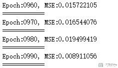
- # 打印与记录误差
- if t%10 == 0:
- print("Epoch:{:0>4d}, MSE:{:<10.9f}".format(t,loss.item()))
- print('============')
- hist[t] = loss.item()
基本都是常规的操作,有两个需要注意一下:
- 不是每次都进行反向传播和系数的优化, 我们会把一个epoch所有的loss求和, 一起进行反向传播.
- 还有一点要注意的是, create_dataset需要写在epoch的循环里面, 可以理解一下为什么.
结果的可视化
在这里我没在测试集上做测试, 就直接看一下训练集的效果。首先看一下预测的值与实际值画的图 :
- # 打印预测和实际
- fig = plt.figure(figsize=(12,7))
- ax = fig.add_subplot(1,1,1)
- ax.plot(pre_output.cpu().detach().numpy(), label="Preds")
- ax.plot(y_train.cpu().detach().numpy(), label="Data")
- ax.legend()
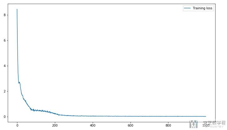
接着看一下训练过程中Loss的变化的过程 :
- # 打印Loss
- fig = plt.figure(figsize=(12,7))
- ax = fig.add_subplot(1,1,1)
- ax.plot(hist, label="Training loss")
- ax.legend()
大概在300个epoch的时候,就已经到较好的效果了。
结语
上面是关于使用Pytorch来实现时间序列的预测,完整的notebook可以参考下面的链接。
- 微信公众号
- 关注微信公众号
-

- QQ群
- 我们的QQ群号
-


2021年1月15日 上午10:37 1F
代码运行到最后导致windows10 企业版 LTSC 死机,为什么?
2021年1月15日 下午5:47 B1
@ 老学生 你需要看一下自己电脑的配置,我是使用 GPU 运行的。可以尝试把 batchsize 调小。
2021年1月15日 下午5:48 B2
@ 王 茂南 不过我感觉数据量不是很大,你是在训练的时候死机吗,是刚开始训练,还是训练了一会。
2021年1月15日 下午6:57 B2
@ 王 茂南 好的,我试试。
2021年1月15日 下午7:20 B2
@ 王 茂南 刚刚在调试状态运行了程序,结果如下:
\anaconda3\lib\site-packages\torch\nn\modules\loss.py:445: UserWarning: Using a target size (torch.Size([])) that is different to the input size (torch.Size([1, 1])). This will likely lead to incorrect results due to broadcasting. Please ensure they have the same size.
return F.mse_loss(input, target, reduction=self.reduction)
程序运行到
Epoch:0510, MSE:0.021993393
============
代码在’loss.backward()’ 处引发异常: bad allocation
Message=bad allocation
Source=F:\MsVsPython\Pytorch\一个初级例子代码\GRUtest\Prj\TrySimplGru\TrySimplGru.py
StackTrace:
File “F:\MsVsPython\Pytorch\一个初级例子代码\GRUtest\Prj\TrySimplGru\TrySimplGru.py”, line 236, in
loss.backward()
是不是那个警告有隐含的错误?我是初学者,不很懂,还请指点!
2021年1月16日 下午3:20 B3
@ 老学生 我一会重新查看一下代码,确认一下是否有问题。
2021年1月15日 下午6:52 2F
好像是训练完成最后显示时死机的
2021年1月16日 下午10:35 B1
@ 老学生 我看了 warning,是 loss 的 target size 和 input size 不同,我在我本地测试了一下,确实会有这个问题,但是不会影响。同时你可以通过 reshape 或者 view 来做改变 target 的大小,这样可以把 warning 去掉。
你可以去这个链接,Notebook 的 Github 链接,有一个 Time Series in PyTorch.ipynb 文件,看一下完整的代码。你可以尝试直接运行这个文件,看一下是否出错。(不过可能是 Pytorch 版本的问题,我的版本是 1.7)。
我看了一下之前写的代码,确实写得比较粗糙,batch size 都是 1,你可以自己调整一下。当时自己就是想做个测试,就没把代码写的比较完善。
2021年1月17日 上午8:57 B2
@ 王 茂南 好的,我试试
2021年1月15日 下午6:55 3F
从博文的结果看好像代码克服了LSTM时序预测平移延迟的现象,不过我现在没有运行到最后,也无法验证,请问你把结果图形放大后确实是这样理想吗?
2021年1月20日 下午4:23 4F
我跑你的jupyter notebook版本,python=3.8.3,pytorch=1.7.1,win10 LTSC 1089,依然出错:
Epoch:0900, MSE:0.025476430
============
—————————————————————————
RuntimeError Traceback (most recent call last)
in
23 # backward
24 loss = loss + criterion(output, j)
—> 25 loss.backward()
26 # optimize
27 optimizer.step()
C:\Anaconda\envs\torch\lib\site-packages\torch\tensor.py in backward(self, gradient, retain_graph, create_graph)
219 retain_graph=retain_graph,
220 create_graph=create_graph)
–> 221 torch.autograd.backward(self, gradient, retain_graph, create_graph)
222
223 def register_hook(self, hook):
C:\Anaconda\envs\torch\lib\site-packages\torch\autograd\__init__.py in backward(tensors, grad_tensors, retain_graph, create_graph, grad_variables)
128 retain_graph = create_graph
129
–> 130 Variable._execution_engine.run_backward(
131 tensors, grad_tensors_, retain_graph, create_graph,
132 allow_unreachable=True) # allow_unreachable flag
RuntimeError: bad allocation
2021年1月21日 上午11:22 B1
@ 老学生 这是内存溢出了。我代码没怎么优化,你可以尝试优化一下。
2021年1月26日 上午8:23 B2
@ 王 茂南 好的
2021年3月18日 下午8:45 5F
forward()里面已经有调用init_hidden()了,在每个batch里面似乎不用再写一遍model.hidden = model.init_hidden()了吧
2021年3月20日 下午12:42 B1
@ ghm 嗯嗯,是的,只需要在 forward 里面写就可以了。