文章目录(Table of Contents)
内容介绍
这一部分主要参考一篇综述(见下), 来总结一下整个CNN的发展史.
Wang, Wei, et al. "Development of convolutional neural network and its application in image classification: a survey." Optical Engineering 58.4 (2019): 040901.
这一篇会主要分为五个部分,分别如下:
- About 2018 ACM A.M. Turing Award
- LeNet
- AlexNet
- VGG16/19
- GoogleNet
- ResNet及一些改进
概述
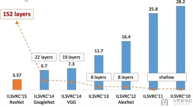
一些经典的CNN在ILSVR比赛中的表现如下,可以看到层数是在递增,同时loss在下降. 后面会详细介绍每一个经典的网络。
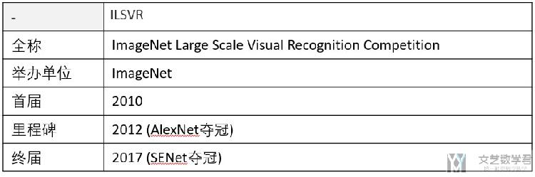
关于ILSVR的一些介绍:
About 2018 ACM A.M. Turing Award
这一部分会首先介绍一下2018年Turing Award的情况, 因为后面讲到的LeNet和AlexNet都会和获奖者有关,所以这里就稍微介绍一下。(Fathers of the Deep Learning Revolution Receive ACM A.M. Turing Award, Bengio, Hinton and LeCun Ushered in Major Breakthroughs in Artificial Intelligence.)
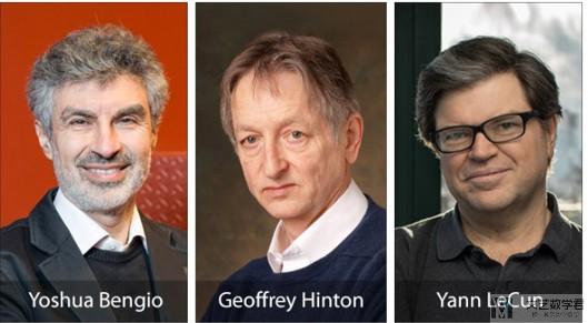
Geoffrey Hinton
- Backpropagation: In a 1986 paper, “Learning Internal Representations by Error Propagation”
- Boltzmann Machines: In 1983, with Terrence Sejnowski, Hinton invented Boltzmann Machines
- Improvements to convolutional neural networks: In 2012, with his students, Alex Krizhevsky and Ilya Sutskever, Hinton improved convolutional neural networks using rectified linear neurons and dropout regularization. In the prominent ImageNet competition, Hinton and his students almost halved the error rate for object recognition and reshaped the computer vision field. (AlexNet)
Yann LeCun
- Convolutional neural networks : In the 1980s, LeCun developed convolutional neural networks
- Convolutional neural networks : In the late 1980s, while working at the University of Toronto and Bell Labs, LeCun was the first to train a convolutional neural network system on images of handwritten digits.
- Improving backpropagation algorithms: LeCun proposed an early version of the backpropagation algorithm (backprop), and gave a clean derivation of it based on variational principles.
- Broadening the vision of neural networks: LeCun is also credited with developing a broader vision for neural networks as a computational model for a wide range of tasks, introducing in early work a number of concepts now fundamental in AI.
Yoshua Bengio
- Probabilistic models of sequences: In the 1990s, Bengio combined neural networks with probabilistic models of sequences, such as hidden Markov models.
- High-dimensional word embeddings and attention: In 2000, Bengio authored the landmark paper, “A Neural Probabilistic Language Model,” that introduced high-dimension word embeddings as a representation of word meaning.
- Generative adversarial networks: Since 2010, Bengio’s papers on generative deep learning, in particular the Generative Adversarial Networks (GANs) developed with Ian Goodfellow, have spawned a revolution in computer vision and computer graphics.
LeNet
LeNet是Yann LeCun在1998年的论文中所提出的, 他是一个经典的CNN的结构,由卷积层,池化层和全连接层构成。(一些具体的评价看下面英文的部分)
Ref : LeCun et al., “Gradient-based learning applied to document recognition,” Proc. IEEE 86(11), 2278–2324 (1998).
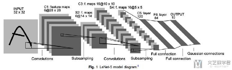
- LeNet-5 is a classical CNN architecture. The combination of convolution layer, pooling layer, and fully connected layer is still the basic components of modern deep CNN.
- LeNet-5 has a groundbreaking significance for the development of deep CNNs.
- Due to insufficient hardware computing and data, LeNet-5 did not attract enough attention after it was proposed.
AlexNet
AlexNet的理论介绍
AlexNet is a milestone in the development of deep CNN, which has caused a new wave of neural network research. (因为AlexNet在ILSVR比赛中取得了较好的成绩, 引发了新的对于CNN的研究的热潮)
与LeNet-5相比, AlexNet的改变有以下的几点:
- ReLU activation function. ReLU can introduce both nonlinearity and sparsity into the network. Sparsity can activate neurons selectively or in a distributed manner. It can learn relatively sparse features and achieve automatic dissociation. (与LeNet相比, 主要的变化, 换了激活函数, 这里使用ReLU作为激活函数)
- Data augmentation. AlexNet uses label-preserving transformations to artificially enlarge the dataset. The form of data augmentation consists of generating image translations, horizontal reflections, and altering the intensities of the RGB channels in training images.(使用了数据增强)
- Dropout. Neurons can be discarded from the network according to a certain probability to reduce network model parameters and prevent overfitting.
- Training on two NVIDIA GTX 580 3GB GPUs. With the development of GPU parallel computing ability, this method speeds up network training.
- Local response normalization (LRN). (Not Common Anymore, 这个方法在VGG的实验中被证明是无效的)
- Overlapping pooling. The pooling step size is smaller than the corresponding edge of pooling kernel. (Overlapping Pooling is the pooling with stride smaller than the kernel size while Non-Overlapping Pooling is the pooling with stride equal to or larger than the kernel size.)
- AlexNet consists of eight layers: five convolutional layers, two fully-connected hidden layers, and one fully-connected output layer. (共有8层)
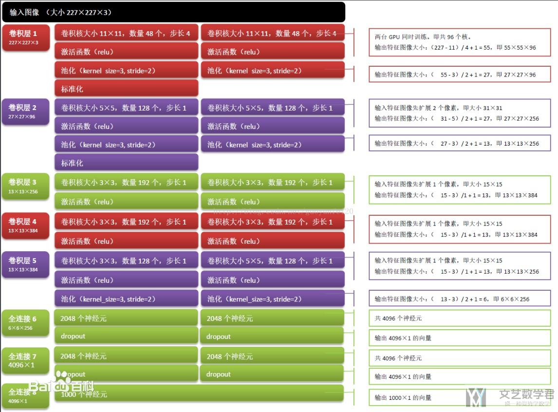
AlexNet的整体结构如下图所示, 在当时因为算力的原因, 使用了两块GPU并行进行计算:
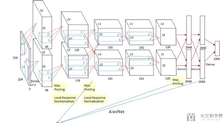
除了箭头指出的三层, 其余上下两个不会互相"影响". 下面的图片是AlexNet详细的参数,原图可以查AlexNet的百度百科. 这个也是使用两个GPU的时候的参数.
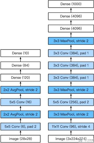
因为目前GPU的提升, 我们可以使用一个GPU来进行计算, 这个时候他的总体结构如下所示(下图左侧是LeNet, 右侧是AlexNet):
AlexNet的Pytorch具体实现
这里只使用Pytorch来实现一下网络的结构, 不包含训练的过程. 为了控制模型的复杂度, 这里在全连接层使用了dropout. 整体的模型结构如下所示:
- net = nn.Sequential(
- nn.Conv2d(1, 96, kernel_size=11, stride=4, padding=1), nn.ReLU(),
- nn.MaxPool2d(kernel_size=3, stride=2),
- nn.Conv2d(96, 256, kernel_size=5, padding=2), nn.ReLU(),
- nn.MaxPool2d(kernel_size=3, stride=2),
- nn.Conv2d(256, 384, kernel_size=3, padding=1), nn.ReLU(),
- nn.Conv2d(384, 384, kernel_size=3, padding=1), nn.ReLU(),
- nn.Conv2d(384, 256, kernel_size=3, padding=1), nn.ReLU(),
- nn.MaxPool2d(kernel_size=3, stride=2),
- nn.Flatten(),
- nn.Dropout(p=0.5),
- nn.Linear(6400, 4096), nn.ReLU(),
- nn.Dropout(p=0.5),
- nn.Linear(4096, 4096), nn.ReLU(),
- nn.Linear(4096, 10))
ZFNet
ZFNet是ILSVR13的冠军,他对AlexNet做了一些小的修改, 主要是讲卷积核的大小变小了。
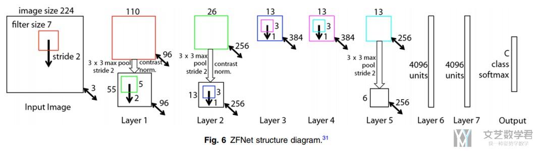
- The network has made minor improvements on AlexNet;
- It changed the size of the convolution kernel in AlexNet's first layer from 11×11 to 7×7. (改变了kernel size)
- It changed the step size of the convolution kernel from 4 to 2. (改变了stride)
Comparing ZFNet model with AlexNet single model, the error rate of top-5 is reduced by 1.7%, which confirms the correctness of this improvement.
VGG16/19
接下来的VGG和GoogleNet就是开始往更深的方向进行发展. 其中VGG有19层, 而GoogLeNet有22层. VGG的全称是:

VGG的网络结构
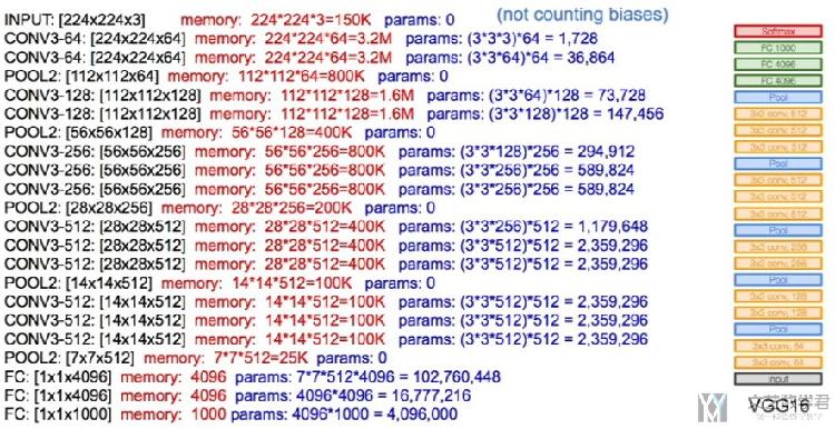
关于VGG网络的整体的结构,如下图所示,其实整体结构与最初的CNN的结构并没有发生很大的变化:
VGG的主要改进
The main contribution of VGG is a thorough evaluation of networks of increasing depth using an architecture with very small (3 × 3) convolution filters, which shows that a significant improvement on the prior-art configurations can be achieved by pushing the depth to 16 to 19 weight layers. (VGG的主要改变是, 通过减小卷积核的大小, 从而来增加网络的深度), 在原文他测试了不同的深度, 最后才有了VGG16/19. 原文名称如下 :
Ref. Simonyan and A. Zisserman, "Very deep convolutional networks for large-scale image recognition," in Int. Conf. Learn. Represent.(2015).
解释--为什么缩小Convolution filter是有效的
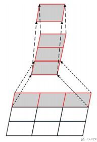
我们注意到VGG的主要改进是使用very small (3 × 3) convolution filters,下面解释一下这样做的可行性.
我们要注意到,两层的3×3的convolutions的视野大小相当于是一层的5×5的convolutions的事业的大小,我们看下面的图. (The receptive field of two 3 × 3 convolutions is equivalent to that of a 5 × 5 convolution and the receptive field of three 3 × 3 convolutions is equivalent to that of a 7 × 7 convolution.)
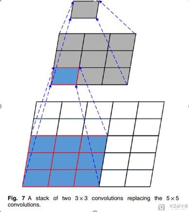
从上面的图中,可以看出,经过两层3×3的convolutions后, 新的单个pixel有原来5×5的视野, 相当于一层3×3的convolutions。这样做可以带来下面的两个的好处 :
- First, it contains three ReLU layers instead of one, making the decision function more discriminatory; (可以经过更多的激活层, 可以更有区分度)
- Second, it can reduce the number of parameters. For example, if the input and output both have C channels, 3 × (3 × 3 × C × C)= 27 × C × C parameters are required for three convolution layers of 3 × 3, and 7 × 7 × C × C =49 × C × C parameters are required for one convolution layer of 7 × 7.(参数减少了, 上面是详细的计算过程)
VGG的结构
在VGG网络中, 作者将CNN的设计表示为由block组成的. 每一个block有以下的部分:
- a convolutional layer (with padding to maintain the resolution)
- a nonlinearity such as a ReLU
- a pooling layer such as a max pooling layer
在原始的VGG中, 由两个部分组成, 分别是全面的卷积以及后面的全连接层. 在卷积层有5个block:
- 前两个block只有一个卷积层. 后面三个block有二个卷积层.
- 第一个block的output channel是64, 后面的输出每次乘2, 直到512.
- 最后VGG是三层的全连接网络.
Pytorch实现VGG具体结构
我们看一下在Pytorch中, 如何简单的实现VGG的结构. 首先我们定义VGG中的block的结构. 简单做一下说明, 一个block可以由多个卷积层组成. 下一个卷积层的in channel是上一个卷积层的out channel.
- def vgg_block(num_convs, in_channels, out_channels):
- layers=[]
- for _ in range(num_convs):
- layers.append(nn.Conv2d(in_channels, out_channels,
- kernel_size=3, padding=1))
- layers.append(nn.ReLU())
- in_channels = out_channels
- layers.append(nn.MaxPool2d(kernel_size=2,stride=2))
- return nn.Sequential(*layers)
例如下面的例子, 我们迭3个卷积层, 初始的input channel是3, output channel是10.
- vgg_block(3,3,10)
- """
- Sequential(
- (0): Conv2d(3, 10, kernel_size=(3, 3), stride=(1, 1), padding=(1, 1))
- (1): ReLU()
- (2): Conv2d(10, 10, kernel_size=(3, 3), stride=(1, 1), padding=(1, 1))
- (3): ReLU()
- (4): Conv2d(10, 10, kernel_size=(3, 3), stride=(1, 1), padding=(1, 1))
- (5): ReLU()
- (6): MaxPool2d(kernel_size=2, stride=2, padding=0, dilation=1, ceil_mode=False)
- )
- """
接着我们将block相叠加, 组成完成的VGG网络.
- def vgg(conv_arch):
- # The convulational layer part
- conv_blks=[]
- in_channels=1
- for (num_convs, out_channels) in conv_arch:
- conv_blks.append(vgg_block(num_convs, in_channels, out_channels))
- in_channels = out_channels
- return nn.Sequential(
- *conv_blks, nn.Flatten(),
- nn.Linear(out_channels*7*7, 4096), nn.ReLU(), nn.Dropout(0.5),
- nn.Linear(4096, 4096), nn.ReLU(), nn.Dropout(0.5),
- nn.Linear(4096, 10))
- net = vgg(conv_arch)
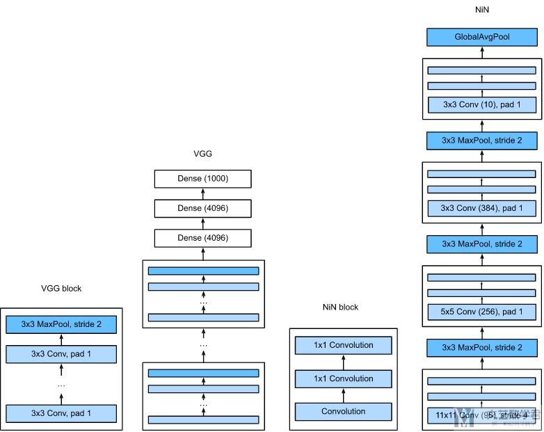
Network in Network (NiN)
上面介绍的AlexNet, VGG等网络都有一个共同的特征, 通过卷积层来提取spatial structure, 接着通过一个全连接层. 但是NiN的想法和之前的不一样, 在经过卷积层之后, 他会通过一个全连接层, 也就是对每一个pixel都进行处理. 在实际实现的时候, 就是使用一个1×1大小的卷积. 下面详细看一下NiN的构造.
NiN的Block
The idea behind NiN is to apply a fully-connected layer at each pixel location (for each height and width). If we tie the weights across each spatial location, we could think of this as a 1×1 convolutional layer or as a fully-connected layer acting independently on each pixel location. Another way to view this is to think of each element in the spatial dimension (height and width) as equivalent to an example and the channel as equivalent to a feature.
也就是说, 在NiN中, 比如现在是3×64×64的图片, 那么我们将其看成64×64个单独的数据, 每个数据有3维的特征, 这时候用1×1的卷积, 就可以对这样特征进行线性组合.
我们看一下使用Pytorch实现NiN的Block.
- def nin_block(in_channels, out_channels, kernel_size, strides, padding):
- return nn.Sequential(
- nn.Conv2d(in_channels, out_channels, kernel_size, strides, padding),
- nn.ReLU(),
- nn.Conv2d(out_channels, out_channels, kernel_size=1), nn.ReLU(),
- nn.Conv2d(out_channels, out_channels, kernel_size=1), nn.ReLU())
如果原始的input channel是3, output channel是3, 那么这个block的构造如下:
- nin_block(3,3,3,1,0)
- """
- Sequential(
- (0): Conv2d(3, 3, kernel_size=(3, 3), stride=(1, 1))
- (1): ReLU()
- (2): Conv2d(3, 3, kernel_size=(1, 1), stride=(1, 1))
- (3): ReLU()
- (4): Conv2d(3, 3, kernel_size=(1, 1), stride=(1, 1))
- (5): ReLU()
- )
- """
我们可以看一下网络的参数个数, 如果卷积大小是3, input channel是3, output channel是3. 于是我们可以将一个卷积相成一个三维的正方体, 每次计算3×3×3大小的位置. 因为output channel是3, 所以有3个这样的正方体, 所以参数个数是3×3×3×3=81个. 注意这里是没有bias的.
- a = nn.Conv2d(3, 3, 3, 1, 0, bias=False)
- sum(p.numel() for p in a.parameters())
- """
- 81
- """
同样看一下卷积大小是1的时候. 和上面的思路类似, 参数计算为1×3×3=9.
- a = nn.Conv2d(3, 3, 1, 1, 0, bias=False)
- sum(p.numel() for p in a.parameters())
- """
- 9
- """
NiN的结构
上面介绍了NiN每一个block的组成细节. 下面看一下NiN整体的结构. 整体结构如下图所示. 每一个block如上面所介绍的, block之间是通过maxpool相连.
最原始的NiN是在AlexNet之后, 很短的一段时间内出来的, 他的网络参数如下:
- 卷积层的kernel size是, 11×11, 5×5, 3×3;
- 每一个NiN Block之后都会接一个maximum pooling layer, stride=2, window size=3;
同时, NiN与AlexNet还有一个很大的不同, 在NiN最后没有使用全连接层. 最后一个NiN Block的output channel的大小与label class的大小相同, 之后接了一个global average pooling, 来产生logits. 这样做的好处是很大程度上减小了参数量.
我们使用nn.AdaptiveMaxPool2d((1,1)来完成最后一层, 这个函数就是说对每一张图片的一个channel, 最后输出大小就是(1,1). 具体的可以看一下下面的例子.
- net = nn.Sequential(
- nin_block(1, 96, kernel_size=11, strides=4, padding=0),
- nn.MaxPool2d(3, stride=2),
- nin_block(96, 256, kernel_size=5, strides=1, padding=2),
- nn.MaxPool2d(3, stride=2),
- nin_block(256, 384, kernel_size=3, strides=1, padding=1),
- nn.MaxPool2d(3, stride=2),
- nn.Dropout(0.5),
- nin_block(384, 10, kernel_size=3, strides=1, padding=1),
- nn.AdaptiveMaxPool2d((1,1)),
- nn.Flatten())
我们打印一下每一层参数的变化. 在最后, 在AdaptiveMaxPool之前, 一个数据大小是10×5×5, 接着AdaptiveMaxPool就是对每一个5×5取最大值, 变为10×1×1, 这样一个数据最终的output大小就是和label个数相同的.
- X = torch.rand(size=(1, 1, 224, 224))
- for layer in net:
- X = layer(X)
- print(layer.__class__.__name__,'output shape:\t', X.shape)
- """
- Sequential output shape: torch.Size([1, 96, 54, 54])
- MaxPool2d output shape: torch.Size([1, 96, 26, 26])
- Sequential output shape: torch.Size([1, 256, 26, 26])
- MaxPool2d output shape: torch.Size([1, 256, 12, 12])
- Sequential output shape: torch.Size([1, 384, 12, 12])
- MaxPool2d output shape: torch.Size([1, 384, 5, 5])
- Dropout output shape: torch.Size([1, 384, 5, 5])
- Sequential output shape: torch.Size([1, 10, 5, 5])
- AdaptiveMaxPool2d output shape: torch.Size([1, 10, 1, 1])
- Flatten output shape: torch.Size([1, 10])
- """
GoogLeNet/Inception v1 to v3
GoogLeNet概述(网络结构)
GoogLeNet达到了22层。下面是GoogLeNet的两个主要的贡献 :
- GoogLeNet broaden the network structure and skillfully proposed the inception module.(他提出了inception module, 一共有三个版本, 后面每个会有介绍, 这个结构的提出使得网络变宽)
- The network with the inception module allowed the model to better describe the input data content while further increasing the depth and width of the network model. (同时, inception module的提出, 还使得网络变深, 使得分类的效果有所提升)

下面我们会分为两个部分来进行介绍,一个是GoogLeNet整体上的变动, 一部分是介绍Inception v1 to v3.
GoogLeNet整体上变动
Global Average Pooling
GoogLeNet将传统的最后一部分的全连接层去掉, 转而使用全面一层的平均值代替(如下图所示), 这样做的好处是减少了参数.
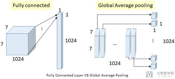
我们可以看一下参数的减少 :
- Number of weights (connections) = 7×7×1024×1024 = 51.3M(使用FC)
- In GoogLeNet, global average pooling is used nearly at the end of network by averaging each feature map from 7×7 to 1×1. Number of weights = 0(使用Average Pooling的时候, 是不需要参数的)
Auxiliary Classifiers for Training
我们可以看到上面GoogLeNet整体结构的时候, 发现他有三个输出, 这些是用作辅助网络的训练, 因为网络的层数较深, 这样做可以用来对抗梯度消失(As we can see there are some intermediate softmax branches at the middle, they are used for training only.)
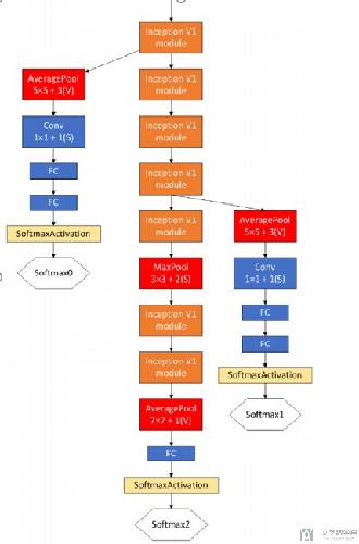
下面是用处的总结 :
- The loss is added to the total loss, with weight 0.3.
- Authors claim it can be used for combating gradient vanishing problem, also providing regularization.(用来对抗梯度消失)
- And it is NOT used in testing or inference time.
Inception v1 to v3
下面介绍Inception Module v1 to v3, 也就是会介绍Inception Blocks的部分.
Inception v1
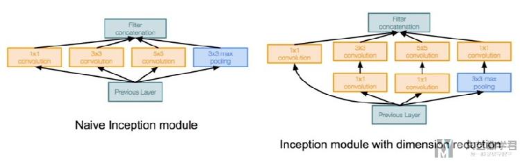
我们使用Inception module来进行网络的扩宽, 如果只是使用Naive Inception Module, 会需要较多的参数, 于是有了Inception module with dimension reduction, 他通过增加1×1的卷积核(bottleneck design), 来减少通道的个数.
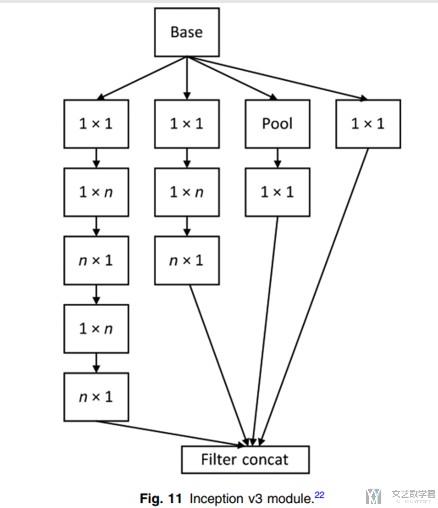
下面这张图是详细的关于Inception Blocks的部分.
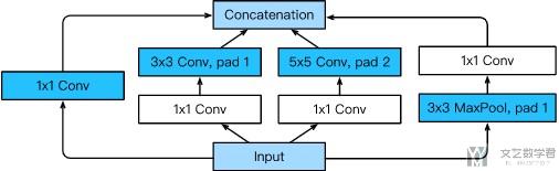
首先我们对Inception Blocks进行简单的介绍.
- 一整个Inception Block有四个独立的通道.
- 前三个通道, 使用不同的卷积核的大小(1×1, 5×5, 3×3), 来提取信息(to extract information from different spatial sizes)
- 中间两个通道, 使用1×1的卷积, 来减少input channel, 来减少模型的复杂度 (后面那我们会讨论参数个数的变化)
- 最后一个通道, 使用3×3最大池化, 接着使用1×1的卷积来改变input channels的数量.
- 这4个通道, 使用padding的方法, 使得4个的输出大小都是一样的
- 最后, 我们将这4个通道的输出, 按照channel进行合并.
接着我们来看一下上面两种Inception Module参数个数的区别。首先是Naive Inception Module :
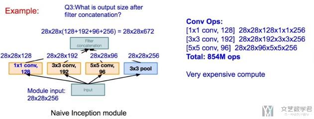
接着是Inception module with dimension reduction,
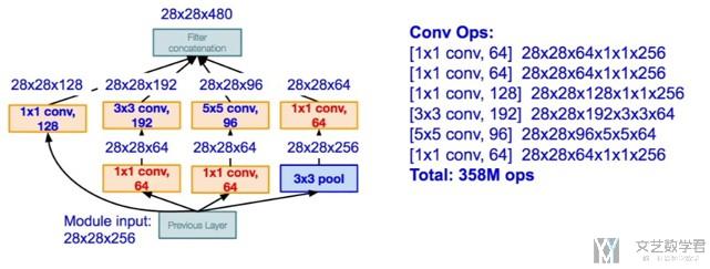
我们可以看到通过增加1×1(bottleneck design)的卷积层(具体如下图所示), 整个module使用的memory减少了一半.
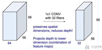
我们总结一下1×1 CONV的特点:
- 图片大小不变
- 压缩filter, 如原始为64, 现在为32
- 每次运算需要的memory变少
- 如对于原始的3×3×192->(28×28×256)×(3×3×192)
- 加入1×1conv后, (28×28×256)×(1×1×64)+(28×28×64)×(3×3×192)
- (28×28)×(3×3×192×256)>(28×28)×(64+3×3×192×64)
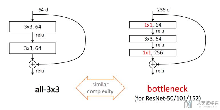
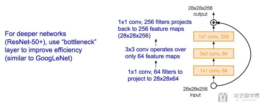
在实际使用的过程中, 可能会出现首先使用1×1的卷积对feature map降维,然后再用3×3的卷积(或其它大小)提取特征,然后再使用1×1的进行升维. 这个想象一下就是很类似与花瓶的形状, 两边宽, 中间小. 下面这张图是在Resnet里面的, 他使用了bottleneck design之后, 增加了网络的层数, 同时还扩大了最后的channel的个数.
关于一些讨论, 可以查看知乎的链接, 深度学习中使用bottleneck design会不会降低模型精度?
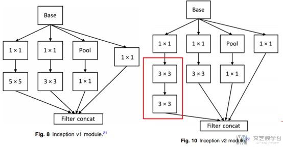
Inception v2
Inception v2主要有下面的两个变化 :
- BN_32 layer is added to normalize the output of each layer to a N (0, 1) Gaussian distribution so that the network can be converges faster and can be initialized more freely.(加入batch normalization)
- In the model, a stack of two 3 × 3 convolution kernels are used to replace 5 × 5 convolution kernels in the inception v1 module, thus increasing the network depth.(将一个5×5拆成两层的3×3, 进一步加深了网络的层数)
Inception v3
关于Inception v3主要有下面的两个变化:
- Spatial factorization into asymmetric convolutions.(使用了非对称的卷积, 如下图所示, 将原来n×n的卷积核变为1×n, n×1两个卷积核, 进一步减少参数, 加深网络)
- The network width has increased, and the network input has changed from 224×224 to 299×299
下面来理解一下非对称卷积:
- 上图中,两层1×3,3×1相当于一层3×3
- 参数减少1/3, 相当于是原来的2/3
- 如input和output的channel为C, 则原来需要3×3×C×C, 现在需要(3×1×C×C)+(1×3×C×C)
GoogleNet的简单代码实现
这里为了方便, 我们就使用Pytorch实现最简单的GoogleNet的结构. 首先我们看一下GoogleNet的总体框架. 总体框架如下图所示, 其中包含9个上面介绍的Inception Block部分.
首先, 关于Inception Block的代码, 关于Inception Block的解释见上面, 其实很简单, 就是有4个单独的通带, 一个input分别通过这4个通道, 经过不同大小的卷积核进行处理, 最后按照channel进行合并:
- class Inception(nn.Module):
- # c1 - c4 are the number of output channels for each layer in the path
- def __init__(self, in_channels, c1, c2, c3, c4, **kwargs):
- super(Inception, self).__init__(**kwargs)
- # Path 1 is a single 1 x 1 convolutional layer
- self.p1_1 = nn.Conv2d(in_channels, c1, kernel_size=1)
- # Path 2 is a 1 x 1 convolutional layer followed by a 3 x 3
- # convolutional layer
- self.p2_1 = nn.Conv2d(in_channels, c2[0], kernel_size=1)
- self.p2_2 = nn.Conv2d(c2[0], c2[1], kernel_size=3, padding=1)
- # Path 3 is a 1 x 1 convolutional layer followed by a 5 x 5
- # convolutional layer
- self.p3_1 = nn.Conv2d(in_channels, c3[0], kernel_size=1)
- self.p3_2 = nn.Conv2d(c3[0], c3[1], kernel_size=5, padding=2)
- # Path 4 is a 3 x 3 maximum pooling layer followed by a 1 x 1
- # convolutional layer
- self.p4_1 = nn.MaxPool2d(kernel_size=3, stride=1, padding=1)
- self.p4_2 = nn.Conv2d(in_channels, c4, kernel_size=1)
- def forward(self, x):
- p1 = F.relu(self.p1_1(x))
- p2 = F.relu(self.p2_2(F.relu(self.p2_1(x))))
- p3 = F.relu(self.p3_2(F.relu(self.p3_1(x))))
- p4 = F.relu(self.p4_2(self.p4_1(x)))
- # Concatenate the outputs on the channel dimension
- return torch.cat((p1, p2, p3, p4), dim=1)
第一部分是于AlexNet是相同的, 我们使用卷积层与global average pooling进行堆叠. 第一部分输出结果是有64个channels.
- b1 = nn.Sequential(nn.Conv2d(1, 64, kernel_size=7, stride=2, padding=3),
- nn.ReLU(),
- nn.MaxPool2d(kernel_size=3, stride=2, padding=1))
接着是第二部分, 使用两个卷积层来进行组成. 首先是使用一个1×1的卷积, output channel也是64. 接着使用一个1×1的卷积, 此时output channel是192, 也就是三倍的64.
- b2 = nn.Sequential(nn.Conv2d(64, 64, kernel_size=1),
- nn.ReLU(),
- nn.Conv2d(64, 192, kernel_size=3, padding=1),
- nn.MaxPool2d(kernel_size=3, stride=2, padding=1))
接着是第三部分, 由两个Inception Block来组成. 对于第一个block, 此时input channel是192, 经过四个通道, 四个通道分别输出是64, 128, 32, 32, 也就是最终是64+128+32+32=256的通道数. 接着是第二个block, 此时输入时256个channel, 四个通道的输出分别是128, 192, 96, 64, 也就是最终的输出的channel个数是128+192+96+64=480. 需要注意的是, 例如第三个通道, 我们首先将通道个数压缩到32个, 接着扩展到96个.
- b3 = nn.Sequential(Inception(192, 64, (96, 128), (16, 32), 32),
- Inception(256, 128, (128, 192), (32, 96), 64),
- nn.MaxPool2d(kernel_size=3, stride=2, padding=1))
接着是第四部分, 是由5个Inception Block来组成的. 他们的output channel分别是:
- 192+208+48+64=512
- 160+224+64+64=512
- 128+256+64+64=512
- 112+288+64+64=528
- 256+320+128+128=832
- b4 = nn.Sequential(Inception(480, 192, (96, 208), (16, 48), 64),
- Inception(512, 160, (112, 224), (24, 64), 64),
- Inception(512, 128, (128, 256), (24, 64), 64),
- Inception(512, 112, (144, 288), (32, 64), 64),
- Inception(528, 256, (160, 320), (32, 128), 128),
- nn.MaxPool2d(kernel_size=3, stride=2, padding=1))
最后是第五部分, 第五部分是由两个Inception Block组成的, 最终的output channel是1024. 接着会经过一个global average pooling layer, 将每一个channel都转换为一个1×1的大小, 也就是一个数据最终会转换为对应的通道个数.
- b5 = nn.Sequential(Inception(832, 256, (160, 320), (32, 128), 128),
- Inception(832, 384, (192, 384), (48, 128), 128),
- nn.AdaptiveMaxPool2d((1,1)),
- nn.Flatten())
最后再使用全连接层, 转换为label的格式. 下面是完整的GoogleNet的网络, 把上面几部分拼接起来即可.
- net = nn.Sequential(b1, b2, b3, b4, b5, nn.Linear(1024, 10))
下面假设是一个96×96大小的图片, 只有一个通道.
- 经过第一部分, 此时输出有64个channels;
- 接着经过第二部分, 此时输出是192个channels;
- 接着经过第三部分, 此时输出是480个channels;
- 接着经过第四部分, 此时输出是832个channels;
- 最后经过第五部分, 此时输出是1024, 最后再将这个1024转换为10, 对应label的个数. 这样就是一个简单的GoogleNet的结构.
- X = torch.rand(size=(1, 1, 96, 96))
- for layer in net:
- X = layer(X)
- print(layer.__class__.__name__,'output shape:\t', X.shape)
- """
- Sequential output shape: torch.Size([1, 64, 24, 24])
- Sequential output shape: torch.Size([1, 192, 12, 12])
- Sequential output shape: torch.Size([1, 480, 6, 6])
- Sequential output shape: torch.Size([1, 832, 3, 3])
- Sequential output shape: torch.Size([1, 1024])
- Linear output shape: torch.Size([1, 10])
- """
ResNet
ResNet的想法和由来
上面的VGG和GoogLeNet通过增加网络深度的方法,使得模型的分类效果变好,那么是否可以继续增加网络的深度呢,实际上是不可以的。
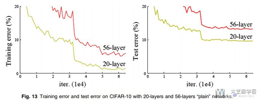
- A problem arises, degradation problems. (从上面的error可以看出, 出现了网络的退化, 更深的网络效果更差)
- This cannot be interpreted as overfitting, as overfit should be better in the training set. The degradation problem shows that deep networks cannot be optimized easily and well. (这个不是overfitting, 因为在training set上结果也不好)
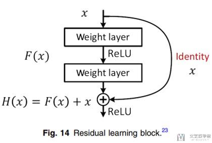
那么有什么办法,可以使得在增加网络深度的情况下,不会出现网络的退化的现象呢。于是ResNet的想法,或是说假设是下面这样的. 他通过设计使用了Residual learning block来达成这样的想法。
The authors argues that stacking layers shouldn't degrade the network performance, because we could simply stack identity mappings (layer that doesn't do anything) upon the current network, and the resulting architecture would perform the same.
This indicates that the deeper model should not produce a training error higher than its shallower counterparts.
于是, ResNet就是由很多个Residual Block来组成的, 如下图所示, 图像来源链接, Review: ResNet — Winner of ILSVRC 2015 (Image Classification, Localization, Detection):

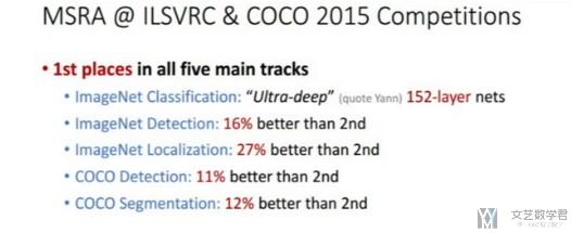
ResNet在当年的各项比赛中均获得了较好的成绩.
理解Residual Block
下图是一个基本的Residual Block, 我们来做一下简单的解释.
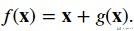
- 假设原来是需要学习的是H(x)
- 现在使用Residual Block时, 则有H(x)=F(x)+x, 相当于要学习F(x)=H(x)-x, 我们可以理解F(x)是网络的残差, 即需要学习的是残差.
- 我们想象, 只需要把Residual Block参数都设置为0,即层数变深变并不会对结果有影响, 输出还是x.
下面是关于Residual Block的详细的介绍:
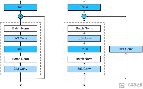
- 每一个Residual Block由两个3×3的卷积组成, 且每一个后面都有BatchNorm和ReLU的激活函数;
- 同时, 作为输入的x, 会直接连接到输出部分, 如果想要改变x的channel, 我们可以通过1×1的卷积来完成;
- 在输出位置, 有一个ReLU函数;
于是, 下面是一个Residual Block的代码:
- class Residual(nn.Module): #@save
- def __init__(self, input_channels, num_channels,
- use_1x1conv=False, strides=1):
- super().__init__()
- self.conv1 = nn.Conv2d(input_channels, num_channels,
- kernel_size=3, padding=1, stride=strides)
- self.conv2 = nn.Conv2d(num_channels, num_channels,
- kernel_size=3, padding=1)
- if use_1x1conv: # 是否对直连的x改变他的channel
- self.conv3 = nn.Conv2d(input_channels, num_channels,
- kernel_size=1, stride=strides)
- else:
- self.conv3 = None
- self.bn1 = nn.BatchNorm2d(num_channels)
- self.bn2 = nn.BatchNorm2d(num_channels)
- self.relu = nn.ReLU(inplace=True)
- def forward(self, X):
- Y = F.relu(self.bn1(self.conv1(X)))
- Y = self.bn2(self.conv2(Y))
- if self.conv3:
- X = self.conv3(X)
- Y += X
- return F.relu(Y)
我们再强调一下, 上面的use_1x1conv=True或是为False的时候, 是两种不同的网络. 如下图所示, 左侧是False的时候, 右侧是True的时候.
在实际使用的时候, 如果我们想要不改变输入图片的通道个数, 那么可以设置use_1x1conv=False. 下面的例子里面, 我们的测试数据是3通道的, 最终的输出结果也是3通道的.
- blk = Residual(3,3)
- X = torch.rand(4, 3, 6, 6)
- Y = blk(X)
- Y.shape
- """
- torch.Size([4, 3, 6, 6])
- """
但是如果我们想要改变输出的通道个数, 此时我们需要设置use_1x1conv=True. 还是上面的例子, 我们输入的通道个数是3, 此时输出的通道个数是8.
- blk = Residual(3,8, use_1x1conv=True, strides=2)
- X = torch.rand(4, 3, 6, 6)
- blk(X).shape
- """
- torch.Size([4, 8, 3, 3])
- """
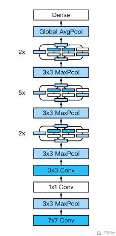
ResNet 18完整网络结构
上面我们介绍了最基本的Residual Block. 下面来看一下组成完成的ResNet. 这里我们用最基本的ResNet来作为例子进行说明, 完整的结构如下所示:
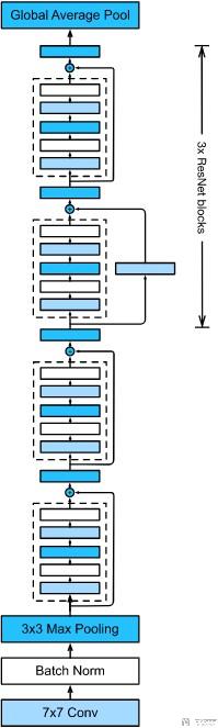
整个网络可以分为三个部分:
- 首先是在网络的输入部分, 会有一个卷积层.
- 接着会接4个大的Residual Block, 每一个大的Residual Block里面会有2个小的Residual Block, 这个就是和我们上面定义的是一样的. 这里共有16个卷积层, 暂时不包含1×1的卷积.
- 最后是输出部分, 这个和之前的GoogleNet也是相同的, 先使用Global Average Block将每个通道的长和宽都转换为1, 接着在通过一个线性层. 这里算是有一层.
所以上面的残差网络又被称为ResNet-18. 下面详细看一下每一部分的代码实现.
首先是第一部分的代码, 包含一个7×7大小卷积核的卷积层, 和一个3×3的maximum pooling layer.
- b1 = nn.Sequential(nn.Conv2d(1, 64, kernel_size=7, stride=2, padding=3),
- nn.BatchNorm2d(64), nn.ReLU(),
- nn.MaxPool2d(kernel_size=3, stride=2, padding=1))
接着是第二部分, 这一部分就是包括4个Residual Block. 每一个里面是由2个小的Block组成的. 因为每一部分都是一样的, 我们可以先定义一个函数来创建这个大的Block. 第一个小的block会对channel有提升, 第二个block的input channel和output channel就是维持不变的.
- def resnet_block(input_channels, num_channels, num_residuals,
- first_block=False):
- blk = []
- for i in range(num_residuals):
- if i == 0 and not first_block: # 第一个block可能需要对channel进行扩充
- blk.append(Residual(input_channels, num_channels,
- use_1x1conv=True, strides=2))
- else: # 后面的block, 输入和输出的channel是相同的.
- blk.append(Residual(num_channels, num_channels))
- return blk
一共有4个block, 下面依次进行创建.
- b2 = nn.Sequential(*resnet_block(64, 64, 2, first_block=True))
- b3 = nn.Sequential(*resnet_block(64, 128, 2))
- b4 = nn.Sequential(*resnet_block(128, 256, 2))
- b5 = nn.Sequential(*resnet_block(256, 512, 2))
最后一部分, 就是一个Global Max Pool和linear. 于是我们将其合成一个整个网络.
- net = nn.Sequential(b1, b2, b3, b4, b5,
- nn.AdaptiveMaxPool2d((1,1)),
- nn.Flatten(), nn.Linear(512, 10))
以上就是一个使用Pytorch实现完整的ResNet-18.
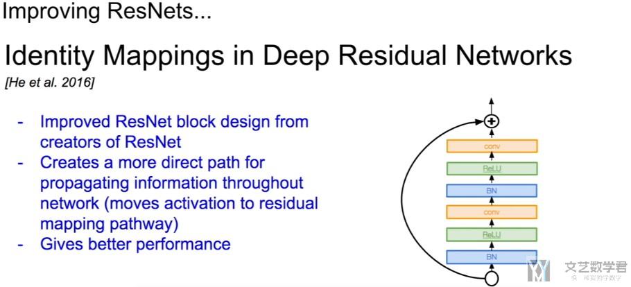
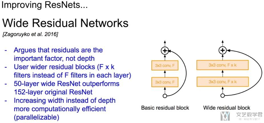
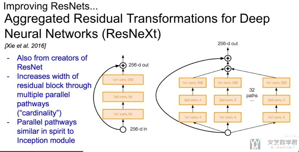
Resdiual Block的一些改进
下面简单罗列一些Resdiual Block的一些改进, 部分就直接放图片, 具体的可以查看相应的论文来进行了解。
Use Bottleneck
与GoogLeNet一样,使用了1×1的卷积核, 使得网络变得更深(上面在讲GoogleNet的时候做了详细的解释).
Identity Mappings in Deep Residual Networks
Wide Residual Networks
ResNeXt
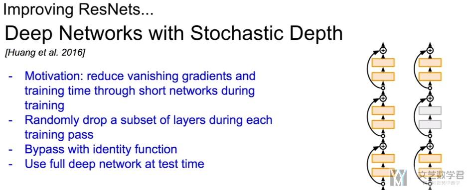
Deep Networks with Stochastic Depth
每一个block有一定可能性被去除, 有些类似Dropout的感觉。
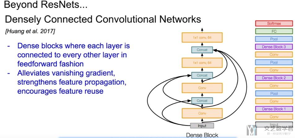
Densely Connected CNN
最后一个介绍的ResNet的改进是Dense Net, 我们首先说一下他的主要的想法. 首先我们看一下对于一个函数来说, 我们可以在某个位置对其进行泰勒展开.

那么其实在ResNet的时候, 我们只进行了一阶的展开. (ResNet decomposes f into a simple linear term and a more complex nonlinear one.)
一些关于Dense Net的其他的优点.
- Connects all layers directly with each other.(这样也可以用来对抗梯度消失的问题)
- In this novel architecture, the input of each layer consists of the feature maps of all earlier layer, and its output is passed to each subsequent layer.
- The feature maps are aggregated with depth-concatenation.
Dense Block的介绍
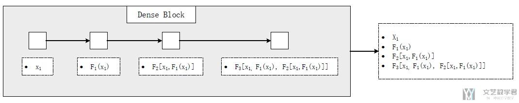
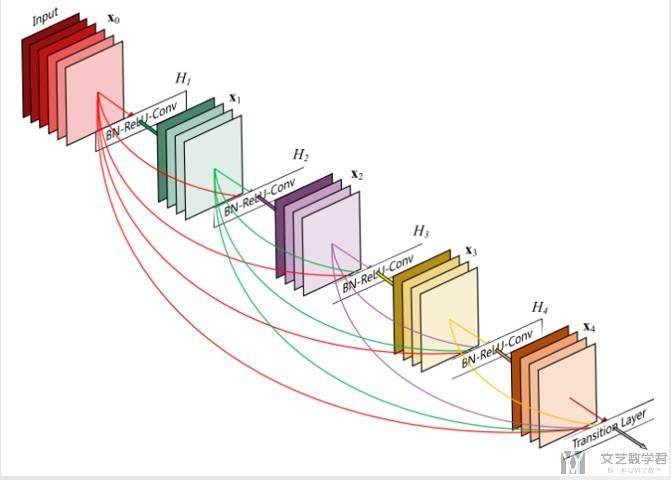
现在在DenseNet里面, 我们希望对其进行高阶的展开, 于是在网络的设计的时候, 我们使用一个Dense Blocks来模拟高阶的值. 下面是一个Dense Block, 里面包含4个卷积.
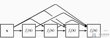
最后的输出不是单纯的相加, 而是将这些值都合并起来. 我们把一个Dense Block的内部具体描述一下. 例如下面, 一个Dense Block会由3个卷积组成:
- 首先是input是x, 经过第一个卷积, 此时输入就是x;
- 在经过第二个卷积的时候, 输入是上一个的输出f(x)和原始的x;
- 以此类推, 前面的所有内容都会用作后面的输入;
- 但是这些输出的channel是一样的, 只有input channel会发生改变.
- 在一个Dense Block结束的时候, 将所有的输出合并起来, 作为一个输出(在channel上进行合并)
下面我们来看一下如何使用Pytorch实现Dense Block. 首先我们实现里面每个小的模块.
- def conv_block(input_channels, num_channels):
- return nn.Sequential(
- nn.BatchNorm2d(input_channels), nn.ReLU(),
- nn.Conv2d(input_channels, num_channels, kernel_size=3, padding=1))
接着, 按照上面的思路, 将小的模块进行组合, 组成一个Dense Block.
- class DenseBlock(nn.Module):
- def __init__(self, num_convs, input_channels, num_channels):
- super(DenseBlock, self).__init__()
- layer = []
- for i in range(num_convs):
- layer.append(conv_block(
- num_channels*i+input_channels, num_channels))
- self.net = nn.Sequential(*layer)
- def forward(self, X):
- for blk in self.net:
- Y = blk(X)
- # Concatenate the input and output of each block on the channel
- # dimension
- X = torch.cat((X, Y), dim=1)
- return X
现在假设里面有4个conv_block, 输入的channel是3, 每一个小的conv_block的output channel是10, 那么一个Dense Block的ouput channel就是3+10×4=43.
- blk = DenseBlock(4, 3, 10)
- X = torch.randn(4, 3, 8, 8)
- Y = blk(X)
- Y.shape
- """
- torch.Size([4, 43, 8, 8])
- """
下面是一个三维的Dense Block的图像.
Transition Layers
每一个Dense Block都会增加channel的个数, 从而增加模型的复杂度. Transition layer的作用就是减少模型的复杂度(A transition layer is used to control the complexity of the model. It reduces the number of channels by using the 1×1 convolutional layer and halves the height and width of the average pooling layer with a stride of 2, further reducing the complexity of the model.)
- def transition_block(input_channels, num_channels):
- return nn.Sequential(
- nn.BatchNorm2d(input_channels), nn.ReLU(),
- nn.Conv2d(input_channels, num_channels, kernel_size=1),
- nn.AvgPool2d(kernel_size=2, stride=2))
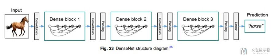
完整的Dense Net
下面是一个完整的Dense Net的结构图. 我们还是使用Pytorch来进行简单的实现.
第一部分还是与之前VGG是一样的, 就是普通的卷积网络.
- b1 = nn.Sequential(
- nn.Conv2d(1, 64, kernel_size=7, stride=2, padding=3),
- nn.BatchNorm2d(64), nn.ReLU(),
- nn.MaxPool2d(kernel_size=3, stride=2, padding=1))
接着是4个Dense Block. 每一个Dense Block之间需要增加transition layer
- num_channels, growth_rate = 64, 32
- num_convs_in_dense_blocks = [4, 4, 4, 4]
- blks = []
- for i, num_convs in enumerate(num_convs_in_dense_blocks):
- blks.append(DenseBlock(num_convs, num_channels, growth_rate))
- # This is the number of output channels in the previous dense block
- num_channels += num_convs * growth_rate
- # A transition layer that haves the number of channels is added between
- # the dense blocks
- if i != len(num_convs_in_dense_blocks) - 1: # 最后一层不需要加
- blks.append(transition_block(num_channels, num_channels // 2))
- num_channels = num_channels // 2
模型的最后部分还是使用Max Pool, 和上面的ResNet等是一样的.
- net = nn.Sequential(
- b1, *blks,
- nn.BatchNorm2d(num_channels), nn.ReLU(),
- nn.AdaptiveMaxPool2d((1,1)),
- nn.Flatten(),
- nn.Linear(num_channels, 10))
我们看一下channel的变化, 使用一个大小为96的数据作为测试.
- X = torch.rand(size=(1, 1, 96, 96))
- for layer in net:
- X = layer(X)
- print(layer.__class__.__name__,'output shape:\t', X.shape)
最终得到的结果如下:
- Sequential output shape: torch.Size([1, 64, 24, 24])
- DenseBlock output shape: torch.Size([1, 192, 24, 24])
- Sequential output shape: torch.Size([1, 96, 12, 12])
- DenseBlock output shape: torch.Size([1, 224, 12, 12])
- Sequential output shape: torch.Size([1, 112, 6, 6])
- DenseBlock output shape: torch.Size([1, 240, 6, 6])
- Sequential output shape: torch.Size([1, 120, 3, 3])
- DenseBlock output shape: torch.Size([1, 248, 3, 3])
- BatchNorm2d output shape: torch.Size([1, 248, 3, 3])
- ReLU output shape: torch.Size([1, 248, 3, 3])
- AdaptiveMaxPool2d output shape: torch.Size([1, 248, 1, 1])
- Flatten output shape: torch.Size([1, 248])
- Linear output shape: torch.Size([1, 10])
我们看一下在Dense Net中, channel的变化.
- 首先在经过第一层的输出时候, output channel是64;
- 接着经过第一个DenseBlock, channel变化为64+32×4=192;
- 接着为了控制channel的个数, channel会除2, 192/2=96;
- 接着经过下一个DenseBlock, channel变化为96+32×4=224;
- 接着又是为了控制channel的个数, channel个数会除2, 224/2=112;
- 后面依此类推,channel的计算都是一样的.
下面一张总结Dense Net.
总结
对于上面的经典的CNN网络,我们使用下面的两张图片进行总结。
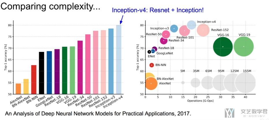
可以看到,随着网络的发展,网络的层数在变深, 同时准确率在上升.
我们接着看一下网络的复杂度和准确率的关系, 可以看到VGG的整体需要的运算量是较大的,之后的网络GoogLeNet一些改进希望减少参数,整体的结果如下图所示。
- 微信公众号
- 关注微信公众号
-

- QQ群
- 我们的QQ群号
-


评论