文章目录(Table of Contents)
传统方法介绍
在Word Embedding使用之前,我们通常会使用1-of-N Encoding的方法对文字进行编码
1-of-N Encoding
所谓,1-of-N Encoding,即每个词汇都是one-hot编码来进行表示。我们来看下面的一个例子。
例子 : 考虑有下面的两句话 :
- Have a good day.
- Have a great day.
这两句话, 共有5个词词汇, 于是可以使用V表示, 其中V = {Have, a, good, great, day}.
因为有5个词汇, 于是每个词汇都用一个5维的向量进行表示, 如下所示 :
Have = [1,0,0,0,0]; a=[0,1,0,0,0] ; good=[0,0,1,0,0]; great=[0,0,0,1,0] ; day=[0,0,0,0,1]`
但这么做有以下的缺点:
- 每个word的vector都是独立的, 所以使用1-of-N Encoding没有体现单词与单词之间的关系;
- 如果词汇量很大, 则vector的维度N会很大, 同时造成数据稀疏问题.
问题本质
其实关于问题本质,相当于是一个无监督的降维的过程,如何能把one-of-encoding的向量转换为一个稠密的向量。
能否使用Auto-Encoder进行训练
那么我们能否使用Auto-Encoder, 答案是不能的。原因如下。
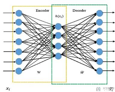
- 在使用Auto-Encoder的时候, input和output是相同的.
- 但是由于Word Vector使用1-of-N Encoding, 每一个Vector都是独立的.
- 这样使用Auto-Encoder是学不到东西的.
如何修改(Word Embedding基本思想)
那么应该如何修改,使得可以获得word vector呢,我们知道Auto-Encoder中input和output是一样的. 那么一个解决办法就是,在word vector中, output是input的下一个词汇,即输入input,来预测下一个词汇.
Word Embedding介绍
我觉得下面这句话来解释Word Embedding很合适: Word embeddings embed meaning of text in a vector space.(把文本的意思嵌入到向量空间中)
想要达到的效果
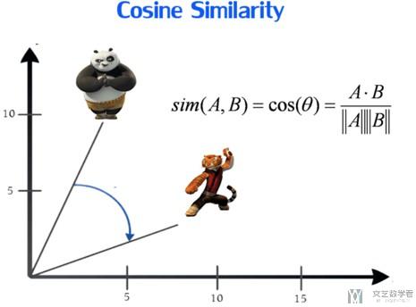
关于word embedding想要达到的效果,我们希望每个word的vector可以表示出语义, 即相似意思的word的vector余弦距离是相接近的.(如我们希望两个意思相近的单词的vector的余弦相似度是1, 即两个vector的夹角越接近0越好)
同时,我们希望每个word的vector是dense vector(稠密向量), 维度会比使用1-of-N Encoding时少很多.
同时,我们希望Word Embedding是unsupervised的, 即我们只有输入的单词,我们就能获得word vector。
一些Word Embedding的方式
下面简单说明以下几种Word Embedding的方法。
- 简单Word Embedding
- 给出前一个词汇, 接着预测后一个词汇.
- 进阶方式
- Word2Vec is one of the most popular technique to learn word embeddings using shallow neural network.
- It was developed by Tomas Mikolov in 2013 at Google.
- Continuous bag if word (CBOW)
- Skip-gram
基本的Word Embedding
参考链接 : Introduction to Word Embedding and Word2Vec
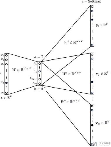
下面简单说明以下基本的Word Embedding的想法。下面的文字主要会来解释这张图片。
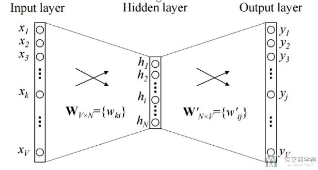
- 关于Input : The input or the context word is a one hot encoded vector of size V.
- 关于Hidden layer(最后这个代表一个word的word vector): The hidden layer contains N neurons.
- 关于Output : The output is again a V length vector with the elements being the softmax values.(用来计算误差)
关于图片中weight的说明
- Wvn is the weight matrix that maps the input x to the hidden layer (V*N dimensional matrix)(其实在这种情况下, Wvn就是最后的word vector, 第一行表示index=1这个单词的vector,因为输入时one hot的)
- W`nv is the weight matrix that maps the hidden layer outputs to the final output layer (N*V dimensional matrix)
需要注意:
There is no activation like sigmoid, tanh or ReLU. The only non-linearity is the softmax calculations in the output layer.
为什么word Embedding能包含语义
我们简单举一个例子,为什么语义接近的单词会在一起(距离接近)。如下面有两句句子:
- 猫是动物.
- 狗是动物.
其中可以看到猫和狗的input是不同的, 但是我们希望output是相同的. 这样就会使得猫, 狗这两个词的word vector距离上是相接近的.
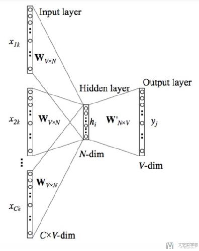
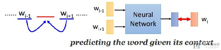
Continuous bag if word(CBOW)
上面我们就使用了前一个词汇去预测后一个词汇,这个想法就是可以使用前n个词汇来预测后一个词汇。(或是使用这个词汇前后n个词汇来预测这个词汇), 网络的结构如下所示。
注意这里输入的C个单词,前面的系数Wvn是一样的,可以简化运算(但是我看别人用Pytorch复现的时候好像设成了不一样的)
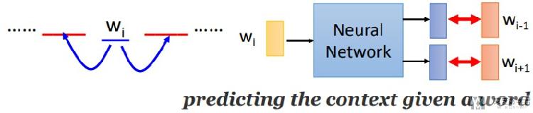
Skip-gram
关于Skip-gram和上面的CBOW有点相反,看网络的结构也能看出来。关于Skip-gram的主要思想是 : 使用目标词汇来预测上下文
Use the target word (whose representation we want to generate) to predict the context and in the process。
CBOW Model V.S Skip-gram
下面简单说一下CBOW和Skip-gram两种方法分别适合什么时候进行使用,并且对两种方法分别进行总结。
- Both have their own advantages and disadvantages.
- According to Mikolov :
- Skip Gram works well with small amount of data and is found to represent rare words well.
- CBOW is faster and has better representations for more frequent words.
CBOW
使用周围的词汇,来预测目标词汇。
Skip-gram
使用目标词汇,来预测上下文。
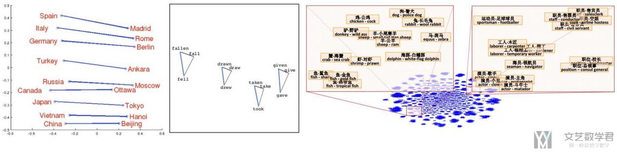
Word Embedding—一些有趣的结果
这一部分是关于Word Embedding的一些有趣的结果。
可以通过简单的逻辑运算,计算单词间的关系; 当然,也可以通过降维后,进行可视化的分析
关于Pytorch中的nn.Embedding功能
之前对于Pytorch中的nn.Embedding能实现的功能一直有一些疑惑。文档中说nn.Embedding是一张查询表, 输入index, 输出vector,那么这个是如何进行训练的(是否使用Skip-Gram或CBOW)
下面是文档中的说明:
Simple lookup table that stores embeddings of a fixed dictionary and size.
This module is often used to store word embeddings and retrieve them using indices. The input to the module is a list of indices, and the output is the corresponding word embeddings.
于是我去Pytorch的论坛上问了以下,不确定答案是否正确吧,但是总之有一个答案。How to implement skip-gram or CBOW in pytorch
一些解释
nn.Embedding可以看成一个优化过的nn.Linear,我们可以看下面的一个例子。
- 假设共有两个词汇, {'Bruce' : 0, 'Wayne' : 1}
- nn.Embedding的weight是[[0.1,0.2,0.3],[0.2,0.5,0.6]]
那么输入单词Wayne(index=1), 输出会是[0.2,0.5,0.6], 代表这个word的vector(相当于右边的矩阵运算)
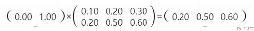
所以, nn.Embedding的weight就是最后的weight。
与nn.Linear的区别
这个也是上面别人的回复,我感觉还是有些道理的,至少能解释通。
In nn.Embeddings back propagation wouldnt happen on the entire matrix. Back propagation will be done only on the rows of the embedding matrix whose indices are passed.
So, less computation is required in this case.
Pytorch实现Skip-Gram
下面简单介绍以下使用Pytorch实现Skip-Gram,前面数据处理的部分就不说了,放一些关键的部分。完整的notebook上传了github,链接如下 : Word Embedding-PyTorch
这里还有一篇别人写的文章,也是使用Pytorch实现word2vector,可以参考一下,Word2Vec in Pytorch - Continuous Bag of Words and Skipgrams
说明 : 可能是数据量太小的原因, 最后word vector的效果并不是很好。
模型的定义
这个也没什么好说的,还是比较简单的。
- class SkipGram(nn.Module):
- def __init__(self, vocab_size, embedding_dim, context_size):
- super(SkipGram, self).__init__()
- self.vocab_size = vocab_size
- self.context_size = context_size
- self.embeddings = nn.Embedding(vocab_size, embedding_dim)
- self.linear1 = nn.Linear(embedding_dim, 128)
- self.linear2 = nn.Linear(128, vocab_size*context_size)
- def forward(self, x):
- # x的大小为, (batch_size, context_size=1, word_index)
- # embedding(x)的大小为, (batch_size, context_size=1, embedding_dim)
- # embeds的大小为, (batch_size, context_size*embedding_dim)
- batch_size = x.size(0)
- embeds = self.embeddings(x).squeeze(1)
- output = F.relu(self.linear1(embeds)) # batch_size*128
- output = F.log_softmax(self.linear2(output),dim=1).view(batch_size, self.vocab_size, self.context_size) # batch * vocab_size*context_size
- output = output.permute(0,2,1)# batch * context_size * vocab_size
- return output
模型的训练
关于模型的训练部分,我们需要关注loss的计算部分。
- # 模型超参数
- NUM_EPOCH = 100
- losses = []
- loss_function = nn.NLLLoss()
- model = SkipGram(lang_process.n_words, embedding_dim=30, context_size=2)
- optimizer = optim.Adam(model.parameters(), lr=0.05)
- exp_lr_scheduler = optim.lr_scheduler.StepLR(optimizer, step_size=10, gamma=0.5)
- # 模型开始训练
- for epoch in range(NUM_EPOCH):
- total_loss = 0
- exp_lr_scheduler.step()
- for num, (trainData, targetData) in enumerate(train_loader):
- # 正向传播
- log_probs = model(trainData)
- # 两次loss分开加
- loss = loss_function(log_probs[:,0,:], targetData[:,0])
- loss = loss + loss_function(log_probs[:,1,:], targetData[:,1])
- # 反向传播
- optimizer.zero_grad()
- loss.backward()
- optimizer.step()
- # Get the Python number from a 1-element Tensor by calling tensor.item()
- total_loss += loss.item()
- losses.append(total_loss)
- if (epoch+1) % 5 == 0:
- print('Epoch : {:0>3d}, Loss : {:<6.4f}, Lr : {:<6.7f}'.format(epoch, total_loss, optimizer.param_groups[0]['lr']))
我们注意到,最后网络会预测前后各一个词汇,所以输出的大小是(batch_size, context_size, vocab_size),最后的target大小是(batch_size, context_size), 这里的context_size就是表示前后两个单词的index,这样是无法直接计算loss的(我暂时还没有想出来), 所以把输出拆成两个,target也拆成两个,大小分别是input : (batch_size, vocab_size), target : (batch_size,) ,这样把两个loss相加即可.
所以上面代码中会有两个loss相加。
关于Skip-gram的实现,主要就是这两个点需要注意。
- 微信公众号
- 关注微信公众号
-

- QQ群
- 我们的QQ群号
-


评论