强化学习的一些应用-入侵检测方向论文

简介

这一篇还是会介绍一下强化学习在实际中的应用. 之前一篇讲过强化学习在控制信号灯上的应用, 强化学习的一些应用-信号灯方向论文. 这一篇主要介绍强化学习在入侵检测, 网络流量检测, 加密流量上的应用. 主要还是以论文介绍为主.

Application of deep reinforcement learning to intrusion detection for supervised problems

这一篇论文, 作者主要使用了不同的强化学习的方法(本文使用了四种强化学习的方法), 来进行入侵检测相关的实验, 并与传统的方法进行了比较. (In this work we present a novel application of several deep reinforcement learning (DRL) algorithms to intrusion detection using a labeled dataset.)

最终得到的结论是, 使用DDQN可以获得比较好的结果, 同时速度比较快.(The conclusion of this comparison is that our proposed framework, using the DDQN algorithm, offers a prediction performance better or similar to the state-of-the-art (SOTA) models, for the two datasets, with the additional advantage of being faster at prediction time.)

本文的创新点

• One important objective for this work is to show that, with some adaptations, we can apply a DRL algorithm using a dataset of labeled samples without interacting with a live environment, as required by the classic DRL framework, and to present in detail the adjustments needed to perform these adaptations. (一个创新点是如何将DL的方法用在入侵检测上, 因为此时我们是无法与环境进行互动的)
• An important result is that the succession of states does not form a sequence since the samples in the dataset are usually independently distributed. This is not the case for classic DRL problems, where the states form a natural sequence and the next state depends on previous states and actions. (这是因为传统的RL的方法, state之间前后只有联系的, 但是在入侵检测的数据中, 前后的样本都是独立的)
• We must take special care with the values of some parameters if we want to obtain good results. Such a parameter is the discount factor, whose value must be very low, contrary to the value that is generally found in classic DRL configurations. (一种简单的处理方法就是将折扣因子, discount factor, 设置得比较小, 这样相当于着重考虑当前得reward, 忽略前后之间得关系.)
• The conclusion of this comparison is that our proposed framework, using the DDQN algorithm, offers a prediction performance better or similar to the state-of-the-art (SOTA) models, for the two datasets, with the additional advantage of being faster at prediction time. (本文使用得方法, DDQN可以获得比较好的实验效果, 同时因为在强化学习里面, 网络比较简单, 所以整体训练的速度是比较快的)

再次总结一下本文的优点, 本文的主要贡献:

• The neural networks used to implement the classifier: Policy, Value or Q functions, are simple and fast, which makes them appropriate for new networks with demanding requirements, such as Internet of Things (IoT) Networks. (RL中网络比较简单, 训练速度快, 可以用在IoT等设备上)
• The resulting neural network is suitable for distributed high-performance computing environments (e.g. Tensorflow); (最后得到的网络可以用在分布式高性能的计算设备上)
•  The reward function used to drive detection can be extremely flexible and does not need to be differentiable. (reward function可以很容易用在不同的检测问题上面)
• The nature of the model allows a simple update of the parameters learned in case of new data available (on-line learning)

本文的相关实验的总体介绍

• 本文主要使用两个数据集, NSL-KDD和AWID.
• 本文所用的四种强化学习的模型, Deep Q-Network (DQN), Double Deep Q-Network (DDQN), Policy Gradient (PG) and Actor-Critic (AC). (这篇文章的模型结构描述很直观, 值得学习)
• 这四种方法会和其他9种模型进行比较, 这9种模型分别是, Support Vector Machine (SVM), Logistic Regression, Naive Bayes (NB), K-Nearest Neighbors (KNN), Random Forest, Gradient Boosting Machine (GBM), AdaBoost, MLP and Convolutional Neural Network (CNN). (这篇文章方法比较时用的图也比较好看, 值得学习)

总共做的实验如下所示:

• NSL-KDD数据集
  • 强化学习模型与其他模型的比较;
  • 强化学习模型中取不同的discount factor对结果的影响;
  • 强化学习模型与其他模型在训练时间上的比较;
• AWID数据集
  • 强化学习模型与其他模型的比较;
  • 强化学习模型中取不同的discount factor对结果的影响;
  • 强化学习模型与其他模型在训练时间上的比较;

本文的数据集介绍

在本文进行的实验中, 选择了两个数据集, 分别是NSL-KDD和AWID. 他选择数据集需要满足下面的7个要求.

• (1) labeled datasets
• (2) unbalanced but with a different level of imbalance, which allows studying the behavior in different conditions (能有不同程度的数据不平衡)
• (3) a predefined split for the training and test sets, which offers a means to compare results from different works (有分好的训练集和测试集)
• (4) well-known datasets, which make available a sufficient number of results from previous works
• (5) to include older and more recent datasets, to increase generality/variability,
• (6) data coming from different network architectures (e.g. fixed-line vs wireless networks), and
• (7) the need to have a data volume large enough to have significant results, but limited by practical restrictions of memory and CPU time.

于是, 对于NSL-KDD数据集来说, 他的主要目的是, verify the capacity of the classifier to handle a different distribution of attacks between the training and test dataset:

• It contains a moderately large number of samples (>120K samples) with continuous and categorical features (>40 features). 数据集有足够数量的样本
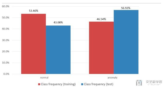
• One interesting aspect of NSL-KDD is that the test and training sets have a different distribution of labels, which is an important challenge for any classifier. 训练集和测试集的label分布是不同的, 这会对分类器造成一定的困难.
• The dataset preparation and scaling for this work is similar to that with the difference that in this case we have aggregated the labels in two categories: normal and anomaly. (简单介绍数据预处理的方法, 这里只进行简单的二分类, normal and anomaly)
• 下图展示了NSL-KDD数据集, 测试集和训练集中数据分布不同. 注意这里只是分布的不同, 但是nromal和anomaly两者的数量差不多. 只不过在训练部分, normal的样本比较多, 在测试集里面, anomaly的样本比较多.

对于AWID来说, 他的主要目的是, verify the ability to handle a very unbalanced dataset.

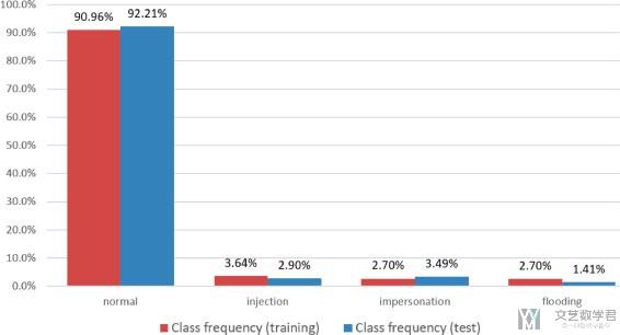
• It has 4 labels to classify: normal, flooding, injection and impersonation; with over 150 categorical and continuous features with a relatively large number of samples for the training (>1,5 M) and test sets (>500 K).
• This dataset is extremely unbalanced with over 90% normal labels. This dataset is more unbalanced than NSL-KDD, but, unlike NSL-KDD, the label distribution for the training and test datasets are quite similar. (样本是非常不平衡的, 大部分的数据都是normal类别的)
• It is also newer and contains more samples than NSL-KDD.
• 下图是AWID数据集的数据分布, 可以看到大部分数据是normal的, 其他label的数据都很少.

数据预处理

为了能适应强化学习的训练, 我们对数据预处理部分进行相关的修改:

• 将network feature看成state;
• 将label value看成action;

整个的获取mini-batches的过程如下, 这个是对应DQN, DDQN和actor-critic算法. Policy gradient会有所不同. 这一篇我们暂时只讲DDQN算法.

• A mini-batch will be a subset of samples drawn at random from the dataset. (一个mini-batch是对整个dataset的随机抽样)
• Each training pass is done with a different mini-batch that is updated by random sampling from the dataset.
• In this case, a mini-batch is formed by n+1 random samples of the dataset.
• Each training iteration of the algorithm will process all the samples of a mini-batch, and for each iteration a new mini-batch is built following the process shown in the above figure.
• The model was trained for 10 epochs, where an epoch is a number of iterations enough to cover the complete dataset. (我们简单概括一下就是, 每一个iteration算法会处理一个mini-batch, 每一个iteration都会生成一个新的mini-batch. 一个epoch是由多个iteration组成的, 且一个epoch会整个dataset里的数据都过一遍. 对应到RL中, 一次iteration相当于是一次模拟, 最后是done, 一个epoch是进行了都次的模拟.)

模型细节介绍

在原文中使用了4中强化学习的模型, 并对这四种模型进行了一一介绍. 我们这里就先着重介绍DDQN和A2C的部分. 其中DDQN也是在实验中获得最好效果的模型. 可以学习一下这里是如何描述模型的, 把数据在模型中的流向绘制的非常清楚.

首先模型DDQN的总体结构如下所示.

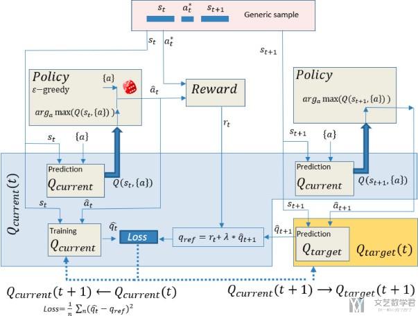
对于上面的结构, 我们进行详细的说明:

• 简单描述一下上面结构的流程, 首先根据data, Q current function返回状态s下不同action的Q值, 再在Policy中根据Q值选择此时的最好的action. 于是此时有了Q(s,a). 同样, 我们对于状态s+1也是计算不同action的Q值, 计算出Q(s+1, a+1), 接着计算loss. (描述的有点简单, 这个就是和DDQN完全一样的, 结合DDQN算法看就能看懂)
• A neural network (NN) is used as a function approximator for the Q Target and Q Current function. We have used a simple NN of 3-layers, with ReLU activation for all layers, including the last one to ensure a positive Q-value. (说明Q function使用的网络结构)
• 关于reward函数的介绍, The reward is a 1/0 reward associated, respectively, to a correct/incorrect prediction. 当我们预测的action和实际的label相同reward就是1, 预测错误reward就是0.
• 这里介绍关于discount factor的选择, 在这里我们要将discout factor设置的比较小. The best performance was obtained by applying a small value for the discount factor (λ). Small values of λ give more importance to learning the current reward, regardless of the succession of future rewards. This makes sense, considering that (1) the next state is uncorrelated with the present state, and (2) we are actually implementing a classifier disguised as a DRL algorithm, being the real goal to make a correct prediction for the current state (current reward).
• 最后当模型训练结束之后, 我们可以使用Q function来进行预测. 输入一个state, 选择返回Q值大的那个action, 也就是最后的预测结果. For a particular state, the Q function will provide a Q-value for each of the possible actions for that state. The predicted action is the one that maximizes the Q-value (no ε-greedy applied for prediction).

下面是模型Actor-Critic模型的介绍, 下面是总体的结构图, 具体的训练细节就是和Actor-Critic是一样的.

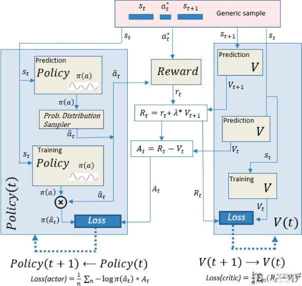
这里需要说明一下, 在预测的时候, 我们就选择概率最大的action即可, 不需要进行sampling. (For prediction, in a similar way to the policy gradient model, we use the NN that implements the policy function, simply by selecting the action with the highest probability (without sampling).)

结果介绍

实验结果介绍部分是按数据集进行划分, 每个里面有三类实验:

• NSL-KDD数据集
  • 强化学习模型与其他模型的比较;
  • 强化学习模型中取不同的discount factor对结果的影响;
  • 强化学习模型与其他模型在训练时间上的比较;
• AWID数据集
  • 强化学习模型与其他模型的比较;
  • 强化学习模型中取不同的discount factor对结果的影响;
  • 强化学习模型与其他模型在训练时间上的比较;

首先是对NSL-KDD数据集, 强化学习模型与其他模型的比较(这个图片比较大, 原图可以查看原始论文). 其中关于传统模型的结果来自Lopez-Martin et al. (2019). (The main results for alternative ML models have been obtained from Lopez-Martin et al. (2019) where the NSL-KDD dataset was applied to several ML models in order to score them.)

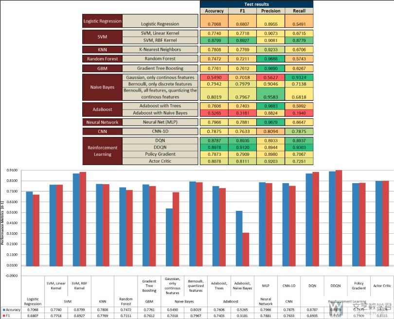
•  The upper part presents the raw data in a color-coded way, where the greenest is associated with a better value and the redder with a worse value (comparison of values is applied column-wise). (上半部分表格的介绍)
• The lower part presents only the accuracy and F1 scores (the most significant scores) in a chart; (下半部分柱状图的介绍)

对于模型结果的一些描述.

• We can observe how the DDQN and DQN models produce the best results (considering F1, accuracy and recall), followed by SVM (with RBF kernel) and actor-critic models.
• We can also observe in Fig. 9 how DDQN stands out in the Recall metric. This metric is very important to guarantee a minimum number of false negatives (samples with an intrusion that are predicted to be normal), which is the main performance metric for an intrusion detection system that tries to identify as many intrusions as possible, considering all of them as critical.

除了比较不同模型之间的性能, 之前提到将RL用在入侵检测上的一个关键就是需要设置较小的discount factor, 于是作者在这里比较了不同大小的discount factor对模型的影响.

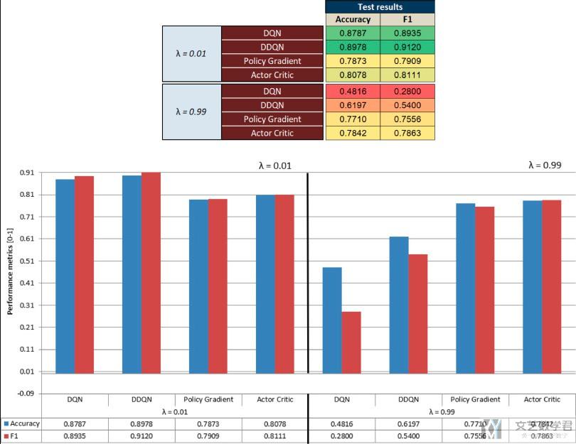
We obtain better results for very low values of the discount factor, as explained in Section 3.2.2.1.

最后是在训练时间上的比较, 强化学习模型与其他模型在训练时长上的比较. 作者在这里比较了训练时间和测试时间. (As presented earlier, one of the advantages of the DRL models is that once trained, the resulting policy function, which provides the correct intrusion label (action) for a specific state (intrusion features), is actually a simple neural network which can be extremely fast for the inference (prediction) stage and, therefore, suitable to be used in an industrial production environment.)

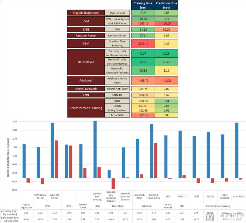
• We can appreciate how the computation times for prediction for the DRL models are really very small compared to the second model with better results (SVM-RBF).
•  Considering the large range of values, the logarithmic scale allows a more suitable view of the data. In the chart of Fig. 11, the smallest values (positive or negative) correspond to a better value in terms of training or prediction times. (因为运行时间差异比较大, 所以可视化的时候取了log)

对于AWID数据集, 同样有强化学习模型与其他模型的比较, 图与上面NSL-KDD部分的类似, 我们就不多介绍了. 同时, 因为AWID是一个多分类的问题, 所以作者在这里给出每一个分类准确率的表格.

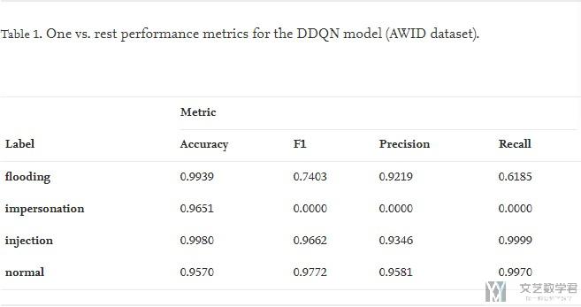
可以看到对于除了impersonation的结果不好, 其他的结果都很好. (Even considering the poor results for one of the class values: impersonation, the rest presents very good results.)

对于为什么impersonation的分类表现不好, 是因为数据集的不同label之间的数量差别很大, 很容易将少类的样本分类的时候都分类为那个占多数的样本. 详细的可以看下面的混淆矩阵. (It is important to keep in mind the strong unbalanced nature of the dataset, and how easy is for a classifier, under these conditions, to adopt the majority class as the unique classification result. This only occurs for one of the class values, impersonation)

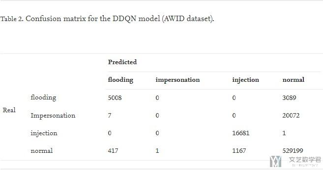
从混淆矩阵可以看到, 几乎所有的impersonation都被分类为normal, 这是因为normal的样本数量是最大的, 所以上面F1值是0, 但是为什么Accuracy这么高呢, 这是因为此时相当于一个二分类问题, 就是impersonation和其他. 虽然没有分对impersonation, 但是也没有其他分到impersonation里面, 在其他的里面的样本数量很多. (The number of true positives in Table 2 is high for all class values except for the impersonation attack, with no true positives, where almost all predictions have fallen within the normal value.)

最后的一些总结:

• The results were obtained with two different IDS datasets, and in both cases our model based on DDQN has been in the set of the best solution models, while the alternative SOTA model, for each dataset, has been very different in each case (SVM and Decision Trees for NSL-KDD and AWID respectively). The conclusion is that our model provides a more robust solution in different scenarios. (在两个数据集中, DDQN都表现很好, 说明该模型有较强的鲁棒性)
• It is particularly important to mention the excellent results of DDQN in the recall metric, which is crucial for an intrusion detection algorithm, since we want to reduce at a minimum the number of false negatives. (DDQN的recall很高)
• In particular, the DDQN model, at test time, provides much smaller prediction times than the best SOTA models studied for this work. (在预测时间上, DDQN也是小很多)
• We can conclude that the application of DRL models to a scenario with a labelled dataset depends to a large extent on the choice of the value of the discount factor. This is an unexpected and significant discovery, since it seems that the fact of not interacting with a live environment (which means that the feedback loop caused by the impact of the actions on the environment is broken), we must be more conservative in each update of our policy function, making the convergence slower but more stable. (对于discount factor来说, 在入侵检测的模型中, 是取值越小越好)