PyTorch快速使用介绍--实现分类

王茂南

2833
文章

75
评论

2018年7月25日09:07:1124 13220字阅读44分4秒

摘要这一篇文章会介绍一个不同激活函数在分类这个网络中的效果，具体来说就是ReLU和Sigmoid两者的效果，并且还会分析一下网络层数的深浅对模型的影响，最后会讲一个扩充数据集的办法。本文会使用PyTorch框架进行实现。

文章目录(Table of Contents)

前言

上一篇文章讲了三种框架来实现线性回归，TensorFlow,Keras,PyTorch框架了解–实现线性回归，这一篇文章会详细介绍一下PyTorch的使用，会使用一个分类的例子来进行介绍。

马上就要是文艺数学君一周年的周年纪念了，到时候看看会有些什么。希望文艺数学君越做越好。

下面就开始正式讲关于PyTorch的内容，我们这次来讲一下分类，上次讲了线性回归，我们的神经网络还是就使用全连接层和激活层来搭建。

这一次介绍的四个模型分别是会比较两种激活函数，ReLU和Sigmoid，模型二和模型三；同时会比较不同层数的区别，模型一与模型二；同时会看一种数据增维的方法，模型四。下面就开始来讲吧。

实现分类

数据准备

我们首先使用sklearn中的datasets生成我们需要的数据；

import numpy as np
from sklearn import datasets
from matplotlib import pyplot as plt
# 生成样例数据
noisy_moons, labels = datasets.make_moons(n_samples=1000, noise=.05, random_state=10) # 生成 1000 个样本并添加噪声
# 其中800个作为训练数据,200个作为测试数据
X_train,Y_train,X_test,Y_test = noisy_moons[:-200],labels[:-200],noisy_moons[-200:],labels[-200:]
print(len(X_train),len(Y_train),len(X_test),len(Y_test))
>> 800 800 200 200

我们可以画图看一下数据的样子：

plt.figure(figsize=(8,6))
plt.scatter(X_test[:,0],X_test[:,1],c=Y_test)

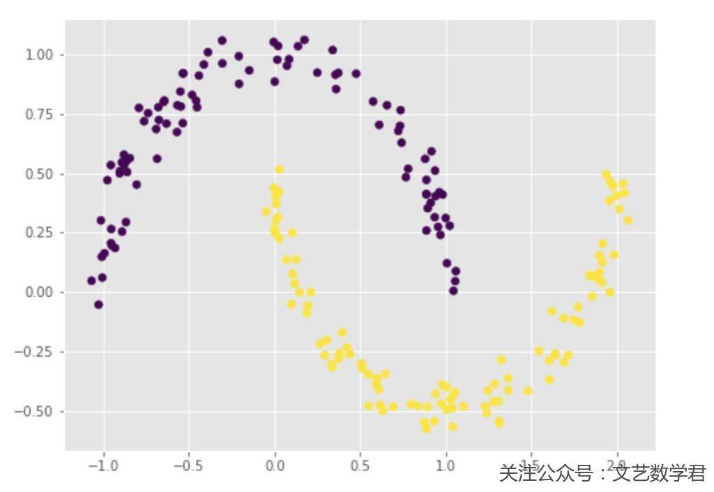
从上面的图像可以看到，我们的数据呈现月牙的形状，这种形状的数据直接使用k-means聚类是不能区分的，下面我们来搭建神经网络来实现以下数据的分类；

我们首先把要使用到的库进行导入：

import torch as t
from torch import nn
from torch import optim
from torch.autograd import Variable
import torch.utils.data as Data
from IPython import display

网络一（使用ReLU作为激活函数、三层）

下面开始介绍第一个模型，由于后面每个模型的代码内容基本差不多，即定义优化器，损失函数，训练绘图那里，就网络定义的地方有点区别，我们就着重先讲网络的结构，后面就贴一下全部的代码：

# ---------
# 网络的定义
# ---------
class classifer(nn.Module):
def __init__(self):
super(classifer, self).__init__()
self.class_col = nn.Sequential(
nn.Linear(2,16),
nn.ReLU(),
nn.Linear(16,16),
nn.ReLU(),
nn.Linear(16,2),
)
def forward(self, x):
out = self.class_col(x)
return out

上面是我们这里使用的网络的结构，输入是2是因为数据有x和y，最后输出也是2是因为分为两类，整个网络一共有三层，下面贴一下完整的代码，注释已经写得很详细了，可以复制下来仔细看一下；

# ----------
# 生成样例数据
# ----------
noisy_moons, labels = datasets.make_moons(n_samples=1000, noise=.05, random_state=10) # 生成 1000 个样本并添加噪声
# 其中800个作为训练数据,200个作为测试数据
X_train,Y_train,X_test,Y_test = noisy_moons[:-200],labels[:-200],noisy_moons[-200:],labels[-200:]
# print(len(X_train),len(Y_train),len(X_test),len(Y_test))
# ---------
# 网络的定义
# ---------
class classifer(nn.Module):
def __init__(self):
super(classifer, self).__init__()
self.class_col = nn.Sequential(
nn.Linear(2,16),
nn.ReLU(),
nn.Linear(16,16),
nn.ReLU(),
nn.Linear(16,2),
)
def forward(self, x):
out = self.class_col(x)
return out
# ----------------
# 定义优化器及损失函数
# ----------------
from torch import optim
model = classifer() # 实例化模型
loss_fn = nn.CrossEntropyLoss() # 定义损失函数
optimiser = optim.SGD(params=model.parameters(), lr=0.05) # 定义优化器
# ------
# 定义变量
# ------
from torch.autograd import Variable
import torch.utils.data as Data
X_train = t.Tensor(X_train) # 输入 x 张量
X_test = t.Tensor(X_test)
Y_train = t.Tensor(Y_train).long() # 输入 y 张量
Y_test = t.Tensor(Y_test).long()
# 使用batch训练
torch_dataset = Data.TensorDataset(X_train, Y_train) # 合并训练数据和目标数据
MINIBATCH_SIZE = 25
loader = Data.DataLoader(
dataset=torch_dataset,
batch_size=MINIBATCH_SIZE,
shuffle=True,
num_workers=2 # set multi-work num read data
)
# ---------
# 进行训练
# ---------
loss_list = []
plt.style.use('ggplot')
for epoch in range(70):
for step, (batch_x, batch_y) in enumerate(loader):
optimiser.zero_grad() # 梯度清零
out = model(batch_x) # 前向传播
loss = loss_fn(out, batch_y) # 计算损失
loss.backward() # 反向传播
optimiser.step() # 随机梯度下降
loss_list.append(loss)
if epoch%10==0:
outputs_train = model(X_train)
_, predicted_train = t.max(outputs_train, 1)
outputs_test = model(X_test)
_, predicted_test = t.max(outputs_test, 1)
# 同时画出训练集和测试的效果
display.clear_output(wait=True)
fig, axes = plt.subplots(nrows=1, ncols=2, figsize=(13,7))
axes[0].scatter(X_train[:,0].numpy(),X_train[:,1].numpy(),c=predicted_train)
axes[0].set_xlabel('train')
axes[1].scatter(X_test[:,0].numpy(),X_test[:,1].numpy(),c=predicted_test)
axes[1].set_xlabel('test')
display.display(fig)

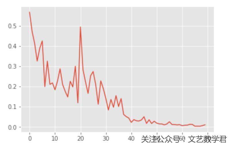
我们来看一下上面代码的输出，左边是训练集上的结果，右边是测试集上的结果：

可以看到最终可以全部分开，我们再看一下loss的情况：

网络二（使用ReLU作为激活函数、五层）

这个网络和上面的区别在于网络层数变深了，我们看一下这时候的情况，还是先看一下网络的定义：

class classifer(nn.Module):
def __init__(self):
super(classifer, self).__init__()
self.class_col = nn.Sequential(
nn.Linear(2,16),
nn.ReLU(),
nn.Linear(16,32),
nn.ReLU(),
nn.Linear(32,32),
nn.ReLU(),
nn.Linear(32,32),
nn.ReLU(),
nn.Linear(32,2),
)
def forward(self, x):
out = self.class_col(x)
return out

和上面的差不多，就是变深了，看一下完整的代码：

# 网路变深
# ----------
# 生成样例数据
# ----------
noisy_moons, labels = datasets.make_moons(n_samples=1000, noise=.05, random_state=10) # 生成 1000 个样本并添加噪声
# 其中800个作为训练数据,200个作为测试数据
X_train,Y_train,X_test,Y_test = noisy_moons[:-200],labels[:-200],noisy_moons[-200:],labels[-200:]
# print(len(X_train),len(Y_train),len(X_test),len(Y_test))
# ---------
# 网络的定义
# ---------
class classifer(nn.Module):
def __init__(self):
super(classifer, self).__init__()
self.class_col = nn.Sequential(
nn.Linear(2,16),
nn.ReLU(),
nn.Linear(16,32),
nn.ReLU(),
nn.Linear(32,32),
nn.ReLU(),
nn.Linear(32,32),
nn.ReLU(),
nn.Linear(32,2),
)
def forward(self, x):
out = self.class_col(x)
return out
# ----------------
# 定义优化器及损失函数
# ----------------
from torch import optim
model = classifer() # 实例化模型
loss_fn = nn.CrossEntropyLoss() # 定义损失函数
optimiser = optim.SGD(params=model.parameters(), lr=0.05) # 定义优化器
# ------
# 定义变量
# ------
from torch.autograd import Variable
import torch.utils.data as Data
X_train = t.Tensor(X_train) # 输入 x 张量
X_test = t.Tensor(X_test)
Y_train = t.Tensor(Y_train).long() # 输入 y 张量
Y_test = t.Tensor(Y_test).long()
# 使用batch训练
torch_dataset = Data.TensorDataset(X_train, Y_train) # 合并训练数据和目标数据
MINIBATCH_SIZE = 25
loader = Data.DataLoader(
dataset=torch_dataset,
batch_size=MINIBATCH_SIZE,
shuffle=True,
num_workers=2 # set multi-work num read data
)
# ---------
# 进行训练
# ---------
loss_list = []
for epoch in range(200):
for step, (batch_x, batch_y) in enumerate(loader):
optimiser.zero_grad() # 梯度清零
out = model(batch_x) # 前向传播
loss = loss_fn(out, batch_y) # 计算损失
loss.backward() # 反向传播
optimiser.step() # 随机梯度下降
loss_list.append(loss)
if epoch%10==0:
outputs = model(X_test)
_, predicted = t.max(outputs, 1)
display.clear_output(wait=True)
plt.style.use('ggplot')
plt.figure(figsize=(12, 8))
plt.scatter(X_test[:,0].numpy(),X_test[:,1].numpy(),c=predicted)
plt.title("epoch: {}, loss:{}".format(epoch+1, loss))
plt.show()

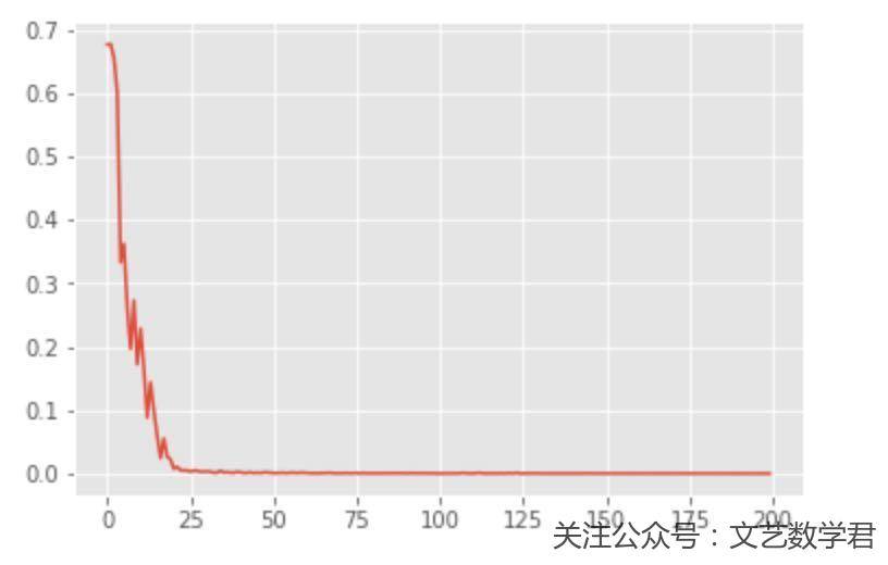
还是看一下训练过程中结果的变化，可以看到收敛还是很快的

接下来可以看一下loss的变化情况，和上面的模型比起来，loss下降更加快了。

网络三（使用Sigmoid作为激活函数、五层）

这个网络我们使用Sigmoid作为激活函数来尝试一下，其他的不变。我们还是先把网络结构打印出来：

# ---------
# 网络的定义
# ---------
class classifer(nn.Module):
def __init__(self):
super(classifer, self).__init__()
self.class_col = nn.Sequential(
nn.Linear(2,16),
nn.Sigmoid(),
nn.Linear(16,32),
nn.Sigmoid(),
nn.Linear(32,32),
nn.Sigmoid(),
nn.Linear(32,32),
nn.Sigmoid(),
nn.Linear(32,2),
)
def forward(self, x):
out = self.class_col(x)
return out

接下来看一下完整的代码：

# 调节网络获得更好的结果
# ----------
# 生成样例数据
# ----------
noisy_moons, labels = datasets.make_moons(n_samples=1000, noise=.05, random_state=10) # 生成 1000 个样本并添加噪声
# 其中800个作为训练数据,200个作为测试数据
X_train,Y_train,X_test,Y_test = noisy_moons[:-200],labels[:-200],noisy_moons[-200:],labels[-200:]
# print(len(X_train),len(Y_train),len(X_test),len(Y_test))
# ---------
# 网络的定义
# ---------
class classifer(nn.Module):
def __init__(self):
super(classifer, self).__init__()
self.class_col = nn.Sequential(
nn.Linear(2,16),
nn.Sigmoid(),
nn.Linear(16,32),
nn.Sigmoid(),
nn.Linear(32,32),
nn.Sigmoid(),
nn.Linear(32,32),
nn.Sigmoid(),
nn.Linear(32,2),
)
def forward(self, x):
out = self.class_col(x)
return out
# ----------------
# 定义优化器及损失函数
# ----------------
from torch import optim
model = classifer() # 实例化模型
loss_fn = nn.CrossEntropyLoss() # 定义损失函数
optimiser = optim.SGD(params=model.parameters(), lr=0.1) # 定义优化器
# ------
# 定义变量
# ------
from torch.autograd import Variable
import torch.utils.data as Data
X_train = t.Tensor(X_train) # 输入 x 张量
X_test = t.Tensor(X_test)
Y_train = t.Tensor(Y_train).long() # 输入 y 张量
Y_test = t.Tensor(Y_test).long()
# 使用batch训练
torch_dataset = Data.TensorDataset(X_train, Y_train) # 合并训练数据和目标数据
MINIBATCH_SIZE = 25
loader = Data.DataLoader(
dataset=torch_dataset,
batch_size=MINIBATCH_SIZE,
shuffle=True,
num_workers=2 # set multi-work num read data
)
# ---------
# 进行训练
# ---------
loss_list = []
for epoch in range(500):
for step, (batch_x, batch_y) in enumerate(loader):
optimiser.zero_grad() # 梯度清零
out = model(batch_x) # 前向传播
loss = loss_fn(out, batch_y) # 计算损失
loss.backward() # 反向传播
optimiser.step() # 随机梯度下降
loss_list.append(loss)
if epoch%10==0:
outputs = model(X_test)
_, predicted = t.max(outputs, 1)
display.clear_output(wait=True)
plt.style.use('ggplot')
plt.figure(figsize=(12, 8))
plt.scatter(X_test[:,0].numpy(),X_test[:,1].numpy(),c=predicted)
plt.title("epoch: {}, loss:{}".format(epoch+1, loss))
plt.show()

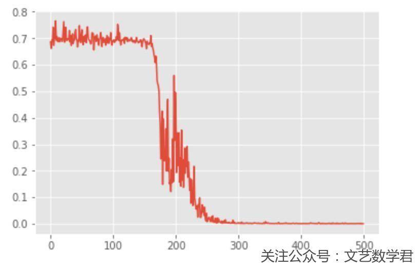
看一下这个训练的动图，可以看到epoch是一直在变化的，前面模型收敛的比较慢：

下面我们看一下loss的图，来看一下上面的想法是否正确：

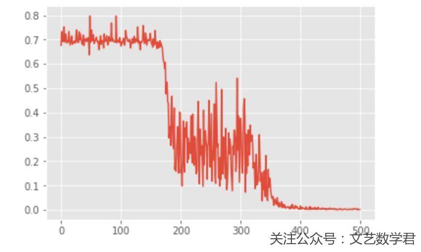
可以看到使用Sigmoid作为激活函数确实会收敛的慢一些，但是也不是所有的都适合用ReLU，有很多情况我也不确定，具体用的时候可以看一下别人写的论文之类的。

网络四（使用Sigmoid作为激活函数、五层、扩充数据集）

这个模型我们会重点介绍一下数据集扩展的方式，我们之前使用的数据集只有两个维度，可以认为是x1和x2，但是有的时候只有这两个数据是不够的，我们可以通过扩充数据集的方式使得模型更快的收敛：

import math
noisy_moons, labels = datasets.make_moons(n_samples=1000, noise=.05, random_state=10) # 生成 1000 个样本并添加噪声
# 增加特征
features1 = (noisy_moons[:,0] * noisy_moons[:,0]).reshape(-1,1)
features2 = (noisy_moons[:,1] * noisy_moons[:,1]).reshape(-1,1)
features3 = (noisy_moons[:,0] * noisy_moons[:,1]).reshape(-1,1)
features4 = np.array([math.sin(i) for i in noisy_moons[:,0]]).reshape(-1,1)
features5 = np.array([math.sin(i) for i in noisy_moons[:,1]]).reshape(-1,1)
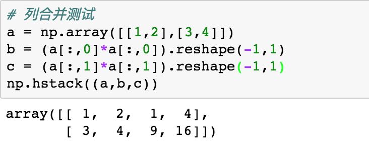
noisy_moons = np.hstack((noisy_moons,features1,features2,features3,features4,features5))

可以看到上面的代码，我们增加了五个特征，x1^2, x2^2, x1*x2, sin(x1)和sin(x1) ,其余的我们不变，还是使用上面的网络结构进行训练，只不过输入要改成7。

我们来看一下上面数据合并的方法，使用一个简单的例子进行查看：

接下来我们来看一下代码：

# 增加特征获得更好的结果
import math
# ----------
# 生成样例数据
# ----------
noisy_moons, labels = datasets.make_moons(n_samples=1000, noise=.05, random_state=10) # 生成 1000 个样本并添加噪声
# 增加特征
features1 = (noisy_moons[:,0] * noisy_moons[:,0]).reshape(-1,1)
features2 = (noisy_moons[:,1] * noisy_moons[:,1]).reshape(-1,1)
features3 = (noisy_moons[:,0] * noisy_moons[:,1]).reshape(-1,1)
features4 = np.array([math.sin(i) for i in noisy_moons[:,0]]).reshape(-1,1)
features5 = np.array([math.sin(i) for i in noisy_moons[:,1]]).reshape(-1,1)
noisy_moons = np.hstack((noisy_moons,features1,features2,features3,features4,features5))
# 其中800个作为训练数据,200个作为测试数据
X_train,Y_train,X_test,Y_test = noisy_moons[:-200],labels[:-200],noisy_moons[-200:],labels[-200:]
# print(len(X_train),len(Y_train),len(X_test),len(Y_test))
# ---------
# 网络的定义
# ---------
class classifer(nn.Module):
def __init__(self):
super(classifer, self).__init__()
self.class_col = nn.Sequential(
nn.Linear(7,32),
nn.Sigmoid(),
nn.Linear(32,32),
nn.Sigmoid(),
nn.Linear(32,32),
nn.Sigmoid(),
nn.Linear(32,32),
nn.Sigmoid(),
nn.Linear(32,2),
)
def forward(self, x):
out = self.class_col(x)
return out
# ----------------
# 定义优化器及损失函数
# ----------------
from torch import optim
model = classifer() # 实例化模型
loss_fn = nn.CrossEntropyLoss() # 定义损失函数
optimiser = optim.SGD(params=model.parameters(), lr=0.1) # 定义优化器
# ------
# 定义变量
# ------
from torch.autograd import Variable
import torch.utils.data as Data
X_train = t.Tensor(X_train) # 输入 x 张量
X_test = t.Tensor(X_test)
Y_train = t.Tensor(Y_train).long() # 输入 y 张量
Y_test = t.Tensor(Y_test).long()
# 使用batch训练
torch_dataset = Data.TensorDataset(X_train, Y_train) # 合并训练数据和目标数据
MINIBATCH_SIZE = 25
loader = Data.DataLoader(
dataset=torch_dataset,
batch_size=MINIBATCH_SIZE,
shuffle=True,
num_workers=2 # set multi-work num read data
)
# ---------
# 进行训练
# ---------
loss_list = []
for epoch in range(500):
for step, (batch_x, batch_y) in enumerate(loader):
optimiser.zero_grad() # 梯度清零
out = model(batch_x) # 前向传播
loss = loss_fn(out, batch_y) # 计算损失
loss.backward() # 反向传播
optimiser.step() # 随机梯度下降
loss_list.append(loss)
if epoch%10==0:
outputs = model(X_test)
_, predicted = t.max(outputs, 1)
display.clear_output(wait=True)
plt.style.use('ggplot')
plt.figure(figsize=(12, 8))
plt.scatter(X_test[:,0].numpy(),X_test[:,1].numpy(),c=predicted)
plt.title("epoch: {}, loss:{}".format(epoch+1, loss))
plt.show()