文章目录(Table of Contents)
简介
之前我们介绍过 Seq2Seq 的模型,Sequence to Sequence Learning with Neural Networks–使用Seq2Seq完成翻译。这一篇文章完成同样的工作,但是我们加上 attention 来完成。
加上 attention 其实就是 pytorch 官网的例子,他就是加上 attention 来进行实现的。TRANSLATION WITH A SEQUENCE TO SEQUENCE NETWORK AND ATTENTION。在这里详细说明一下这个例子。
这一篇还参考下面的链接:
更多参考资料
关于更多 Attention 的资料,可以参考下面的两个链接,这两个链接是论文的复现
- The Annotated Encoder Decoder-A PyTorch tutorial implementing Bahdanau et al. (2015)
- The Annotated Transformer
下面链接是使用 Attention 做的另外一个应用,理解表情的含义。
Seq2Seq with Attention介绍
关于 Attention 的解释,可以看一下这一篇文章, Attention and Memory in Deep Learning and NLP,我在下面简单说一下。
粗略理解 Attention 机制
In the picture above, "Echt", "Dicke" and "Kiste" words are fed into an encoder, and after a special signal (not shown) the decoder starts producing a translated sentence. The decoder keeps generating words until a special end of sentence token is produced. Here, the h vectors represent the internal state of the encoder. (Seq2Seq 简单说明)
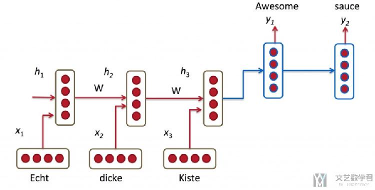
Still, it seems somewhat unreasonable to assume that we can encode all information about a potentially very long sentence into a single vector and then have the decoder produce a good translation based on only that. (Seq2Seq 不合理的地方,将一句话的信息全部压缩到一个向量里面去)
Let's say your source sentence is 50 words long. The first word of the English translation is probably highly correlated with the first word of the source sentence. But that means decoder has to consider information from 50 steps ago, and that information needs to be somehow encoded in the vector. (有的时候句子很长, 只靠vector是不够的)
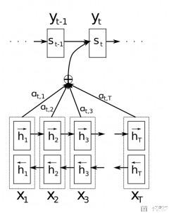
We allow the decoder to "attend" to different parts of the source sentence at each step of the output generation. Importantly, we let the model learn what to attend to based on the input sentence and what it has produced so far. (解决办法, 我们使得 decode 可以得到 encoder 的每一个输出, 让他自己决定各使用多少权重)
The important part is that each decoder output word y_t now depends on a weighted combination of all the input states, not just the last state. (核心思想,decoder 可以将 encoder 部分的 state 加权组合来进行使用)
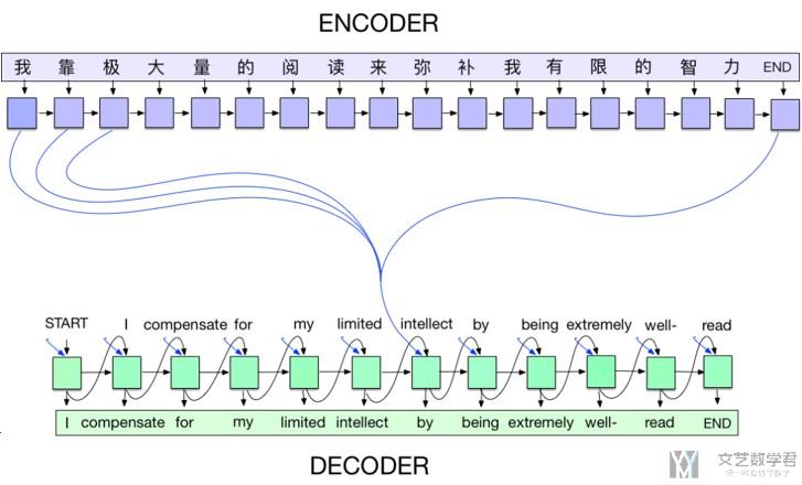
A big advantage of attention is that it gives us the ability to interpret and visualize what the model is doing. For example, by visualizing the attention weight matrix when a sentence is translated, we can understand how the model is translating. (同时,Attention 的一个好处是可以看到生成每个词的时候,模型在关注输入的哪个部分,也就是可以对模型给出解释)
进一步理解 Attention
下面是一些我的想法,结合了上面的一些内容。我们在没有加入 Attention 的时候,整个句子的输入最后就使用 encoder 的一个 state 来表示(只使用了 encoder_hidden 而没有使用 encoder_output),浪费了很多信息,也没有考虑生成的词与前面输入的词的对应关系。
就用翻译来举一个例子,如果 "i am a boy"->"我是男孩",其中「I」应该和「我」的关系是比较大的。所以我们希望在 decoder 的时候, 「I」的输出的权重高一些。于是就有了下面最简单的 Attention 的想法。
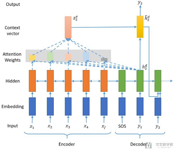
我们在decode输入的时候,不仅有单词的embedding,还有前面encoder的输出乘上权重。如下图所示:
关于 Attention Weight 的权重的计算,我们可以直接将embedding和hidden state合并在一起,再经过一个全连接网络,输出的就是权重(具体可以看一下下面decode的实现)
Attention 模型的实现
因为要处理的事情是一样的,在这里我们就不写数据处理的部分了。数据处理见Sequence to Sequence Learning with Neural Networks–使用Seq2Seq完成翻译。我们主要实现网络的部分。
Encoder部分的网络
Encoder 部分,与没有 Attention 的时候是一样的。将每一个 word 依次输入网络,每个 word 都会有一个 output 和 hidden state。使用前一个单词的 hidden state 作为下一个单词的 hidden state。
The encoder of a seq2seq network is a RNN that outputs some value for every word from the input sentence. For every input word the encoder outputs a vector and a hidden state, and uses the hidden state for the next input word.
- class EncoderRNN(nn.Module):
- def __init__(self, input_size, hidden_size, batch_size=1, n_layers=1):
- super(EncoderRNN, self).__init__()
- self.input_size = input_size
- self.hidden_size = hidden_size
- self.batch_size = batch_size # 输入的时候batch_size
- self.n_layers = n_layers # RNN中的层数
- self.embedding = nn.Embedding(self.input_size, self.hidden_size)
- self.gru = nn.GRU(self.hidden_size, self.hidden_size)
- def forward(self, x):
- self.sentence_length = x.size(0) # 获取一句话的长度
- embedded = self.embedding(x).view(self.sentence_length, 1, -1) # seq_len * batch_size * word_size
- output = embedded
- self.hidden = self.initHidden()
- output, hidden = self.gru(output, self.hidden)
- return output, hidden
- def initHidden(self):
- return torch.zeros(self.n_layers, self.batch_size, self.hidden_size).to(device)
Decoder with Attention
下面是加上 Attention 的 Decode 的部分(这个是核心的部分)。 整个 Decoder 的结构如下所示。其中橘红色的代表变量,蓝色的代表是需要网络层(需要有参数要学习的)。
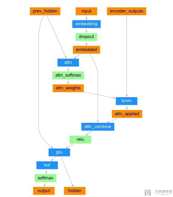
我们做一下简单的解释,解释以下变量大小和具体的步骤。首先有以下的注意:
encoder_outputs 是 encoder 在每一步的输出。也就是说,如果在 encoder 中一次输入十个单词, encoder_outputs 的大小为 (10, feature_size)(这里有点类似的 key 和 value,后面 query 需要和 key 计算相似度)。
权重的计算,是将上一层的 hidden_state 和这一层的 input 拼接起来,过一个全连接层。输出大小为句子长度。比如上面 encoder 是 10 个单词,这里输出大小就是 10,相当于对应上面 10 个 encoder 的输出的权重。这个对应下面的步骤。
- attn_weights = torch.cat((embedded[0],hidden[0]),1)
- attn_weights = self.attn(attn_weights)
- attn_weights = F.softmax(attn_weights,dim=1)
我们再将 attention+embedding 的值合并,作为输入,过一个全连接层再输入 RNN 中。对应下面的步骤:
- output = torch.cat((embedded[0],attn_applied[0]),1)
- output = self.attn_combine(output).unsqueeze(0)
下面是过 RNN,最后就是计算 hidden state 和 output,再输入下一个词汇。
- output, hidden = self.gru(output, hidden)
下面是完整的 decoder 的代码。 每一步的理解可以看上面的过程。
- class AttenDecoder(nn.Module):
- def __init__(self, hidden_size, output_size, dropout_p=0.1, max_length=MAX_LENGTH):
- super(AttenDecoder, self).__init__()
- self.hidden_size = hidden_size
- self.output_size = output_size
- self.dropout_p = dropout_p
- self.max_length = max_length
- self.embedding = nn.Embedding(self.output_size, self.hidden_size)
- self.attn = nn.Linear(self.hidden_size*2, self.max_length)
- self.attn_combine = nn.Linear(self.hidden_size*2, self.hidden_size)
- self.dropout = nn.Dropout(self.dropout_p)
- self.gru = nn.GRU(self.hidden_size, self.hidden_size)
- self.out = nn.Linear(self.hidden_size, self.output_size)
- def forward(self, x, hidden, encoder_outputs):
- # x是输入, 这里有两种类型
- # hidden是上一层中隐藏层的内容
- # encoder_outputs里面是encoder的RNN的每一步的输出(不是最后一个的输出)
- embedded = self.embedding(x).view(1,1,-1)
- embedded = self.dropout(embedded)
- # print('embedded.shape',embedded.shape)
- # ----------------------------
- # 下面的attention weight表示:
- # 连接输入的词向量和上一步的hide state并建立bp训练,
- # 他们决定了attention权重
- # -----------------------------
- attn_weights = torch.cat((embedded[0],hidden[0]),1)
- # print('attn_weights1',attn_weights.shape)
- attn_weights = self.attn(attn_weights)
- attn_weights = F.softmax(attn_weights,dim=1)
- # print('attn_weights2',attn_weights.shape)
- # 这是做矩阵乘法
- # 施加权重到所有的语义向量上
- attn_applied = torch.bmm(attn_weights.unsqueeze(0), encoder_outputs.unsqueeze(0))
- # print('attn_applied',attn_applied.shape)
- # 加了attention的语义向量和输入的词向量共同作为输
- # 此处对应解码方式三+attention
- output = torch.cat((embedded[0], attn_applied[0]),1)
- # print('output1',output.shape)
- # 进入RNN之前,先过了一个全连接层
- output = self.attn_combine(output).unsqueeze(0)
- # print('output2',output.shape)
- output = F.relu(output)
- output, hidden = self.gru(output, hidden)
- # print('output3',output.shape)
- # 输出分类结果
- output = F.log_softmax(self.out(output[0]),dim=1)
- # print('output4',output.shape)
- return output, hidden, attn_weights
模型的训练
上面就是关于 decoder 的定义。下面是在训练的时候还有一些与之前讲的 Seq2Seq 不一样。因为这里 decoder 需要 encoder 全部的 output。
首先我们要处理以下encoder_output,把他处理成长度是一样的。这里没有做padding.
- encoder_output, encoder_hidden = encoder1(input_tensor.unsqueeze(1))
- # 因为一个Decoder的MAX_LENGTH是固定长度的, 所以我们需要将encoder_output变为一样长的
- encoder_output = encoder_output.squeeze(1)
- encoder_outputs = torch.zeros(max_length, encoder_output.size(1)).to(device)
- encoder_outputs[:encoder_output.size(0)] = encoder_output
接下来就是将单词一次输入decoder, 这里还是分为两种模式。
- # Decoder
- loss = 0
- decoder_hidden = encoder_hidden # encoder最后的hidden作为decoder的hidden
- decoder_input = torch.tensor([[SOS_token]]).to(device)
- # 判断是使用哪一种模式
- use_teacher_forcing = True if random.random() < teacher_forcing_ratio else False
- if use_teacher_forcing:
- # Teacher forcing: Feed the target as the next input
- for di in range(target_length):
- decoder_output, decoder_hidden, attn_weights = decoder(decoder_input, decoder_hidden, encoder_outputs)
- loss = loss + criterion(decoder_output, target_tensor[di])
- decoder_input = target_tensor[di] # Teacher Forcing
- else:
- # Without teacher forcing: use its own predictions as the next input
- for di in range(target_length):
- decoder_output, decoder_hidden, attn_weights = decoder(decoder_input, decoder_hidden, encoder_outputs)
- topv, topi = decoder_output.topk(1)
- decoder_input = topi.squeeze().detach() # detach from history as input
- loss = loss + criterion(decoder_output, target_tensor[di])
- if decoder_input.item() == EOS_token:
- break
下面是完整代码。
- teacher_forcing_ratio = 0.5 # 50%的概率使用teacher_forcing的模式
- def train(input_tensor, target_tensor, encoder, decoder, encoder_optimizer, decoder_optimizer, criterion, max_length=MAX_LENGTH):
- encoder_optimizer.zero_grad()
- decoder_optimizer.zero_grad()
- input_length = input_tensor.size(0)
- target_length = target_tensor.size(0)
- # encoder_outputs = torch.zeros(max_length, encoder.hidden_size).to(device)
- # Encoder
- encoder_output, encoder_hidden = encoder1(input_tensor.unsqueeze(1))
- # 因为一个Decoder的MAX_LENGTH是固定长度的, 所以我们需要将encoder_output变为一样长的
- encoder_output = encoder_output.squeeze(1)
- encoder_outputs = torch.zeros(max_length, encoder_output.size(1)).to(device)
- encoder_outputs[:encoder_output.size(0)] = encoder_output
- # Decoder
- loss = 0
- decoder_hidden = encoder_hidden # encoder最后的hidden作为decoder的hidden
- decoder_input = torch.tensor([[SOS_token]]).to(device)
- # 判断是使用哪一种模式
- use_teacher_forcing = True if random.random() < teacher_forcing_ratio else False
- if use_teacher_forcing:
- # Teacher forcing: Feed the target as the next input
- for di in range(target_length):
- decoder_output, decoder_hidden, attn_weights = decoder(decoder_input, decoder_hidden, encoder_outputs)
- loss = loss + criterion(decoder_output, target_tensor[di])
- decoder_input = target_tensor[di] # Teacher Forcing
- else:
- # Without teacher forcing: use its own predictions as the next input
- for di in range(target_length):
- decoder_output, decoder_hidden, attn_weights = decoder(decoder_input, decoder_hidden, encoder_outputs)
- topv, topi = decoder_output.topk(1)
- decoder_input = topi.squeeze().detach() # detach from history as input
- loss = loss + criterion(decoder_output, target_tensor[di])
- if decoder_input.item() == EOS_token:
- break
- # 反向传播, 进行优化
- loss.backward()
- encoder_optimizer.step()
- decoder_optimizer.step()
- return loss.item() / target_length
模型的验证--可视化 Attention
关于模型的训练,查看之前的链接,Sequence to Sequence Learning with Neural Networks–使用Seq2Seq完成翻译,这里就不重复写了。或是可以直接查看文末的代码链接。
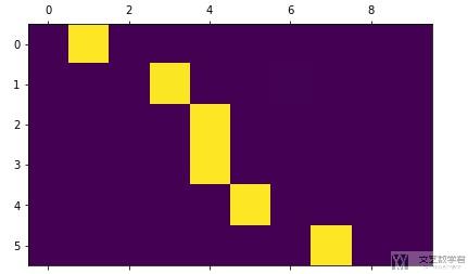
我们这里注意以下如何可视化Attention,其实就是将输入每个word的时候计算出的attention_weight来打印出来。我们注意到上面写AttenDecoder的时候,是由return attenwights的。所以最简答的方式就可以像下面这样进行输出。
- _, attentions = evaluate(encoder1, decoder1, "je suis trop froid .")
- plt.matshow(attentions.cpu().numpy())
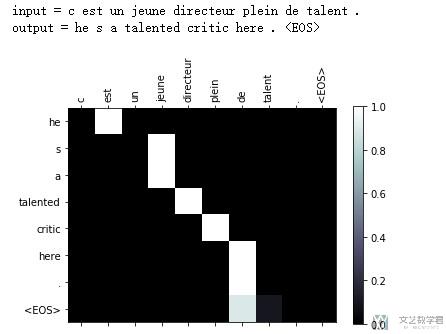
或是我们可以将图画的好看一些,可以使用下面的方式进行实现。(函数来源与Pytorch的官方教程)
- # 更好的可视化
- def showAttention(input_sentence, output_words, attentions):
- # Set up figure with colorbar
- fig = plt.figure()
- ax = fig.add_subplot(111)
- cax = ax.matshow(attentions.numpy(), cmap='bone')
- fig.colorbar(cax)
- # Set up axes
- ax.set_xticklabels([''] + input_sentence.split(' ') +
- ['<EOS>'], rotation=90)
- ax.set_yticklabels([''] + output_words)
- # Show label at every tick
- ax.xaxis.set_major_locator(ticker.MultipleLocator(1))
- ax.yaxis.set_major_locator(ticker.MultipleLocator(1))
- plt.show()
- def evaluateAndShowAttention(input_sentence):
- output_words, attentions = evaluate(encoder1, decoder1, input_sentence)
- print('input =', input_sentence)
- print('output =', ' '.join(output_words))
- showAttention(input_sentence, output_words, attentions)
我们来看一下最终的效果。
- evaluateAndShowAttention("c est un jeune directeur plein de talent .")
到这里,全部的关于attention实现翻译的内容就已经完成了。下面是notebook的链接。
- 微信公众号
- 关注微信公众号
-

- QQ群
- 我们的QQ群号
-


评论