Pytorch入门教程11-Softmax 函数和交叉熵

简介

这一篇我们会讲解二分类问题和多分类问题。在「二分类问题」中，我们可以使用 Sigmoid 作为输出， 看成是一类的概率，另一类的概率就是 1-Sogmoid 的输出结果。但是在多分类问题中，我们需要每一类的概率，这个就需要使用 Softmax。

参考资料

• 关于交叉熵的原理介绍: 熵, 交叉熵, 和KL散度
• 关于 Pytorch 中 CrossEntropyLoss 的介绍: PyTorch中交叉熵的计算-CrossEntropyLoss介绍
• 关于下面 Softmax 的图片来源: Deep Learning — Logistic Classification — using Softmax function
• 一个特别好的文章, Understanding softmax and the negative log-likelihood

关于 Softmax 和多分类问题

Softmax 函数介绍

在多分类问题中，我们需要对每一个类别输出概率，同时要保证这些概率和是 1。这个时候就需要使用 Softmax 函数了。

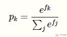
假设现在的输出是 vi（这是一个向量），那么每一个对应 softmax 之后的输出如下：

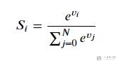
在这里对输入进行指数化，这样可以使得两个输入之间的差距可以扩大。

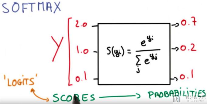
下面我们看一个 softmax 的例子，并使用 Pytorch 中自带的函数进行测试。

下面看一下使用 Pytorch 的测试结果：

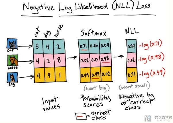
对于多组数据来说，其实 softmax 做的就是将一个矩阵的值压缩到 0 到 1 之间。例如下面的例子，测试数据有三类：

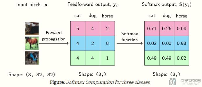
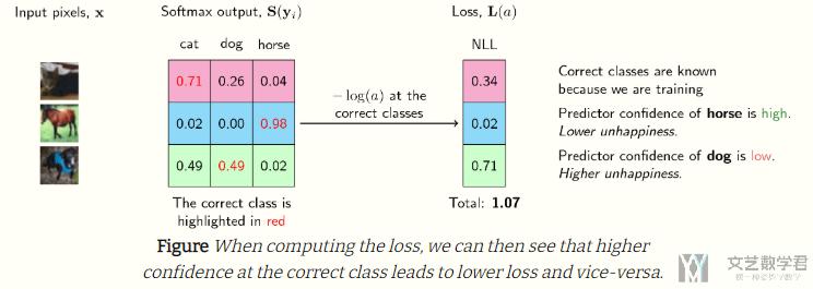
The output of the softmax describes the probability (or if you may, the confidence) of the neural network that a particular sample belongs to a certain class.

Thus, for the first example above, the neural network assigns a confidence of 0.71 that it is a cat, 0.26 that it is a dog, and 0.04 that it is a horse. The same goes for each of the samples above.

交叉熵损失函数

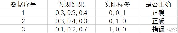
在介绍交叉熵损失函数之前，我们首先看一个例子。现在有一个三分类的问题，一共有三个测试数据，两个测试的模型，他们的结果分别如下所示：

模型一的结果：

模型二的结果：

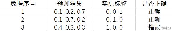
• 对于两个模型的准确率来说，是一样的，准确率都是 2/3；
• 对于「模型一」来说，他在数据 1 和数据 2 上，对结果的确定性都不是很确定，都是 0.4，只比 0.3 大一点；
• 对于「模型二」来说，他的预测结果就表现很肯定，对结果的可能性都是 0.7，会远远比其他类别要大。

所以可以看到，虽说上面两个模型在准确率上的表现是一样的，但是实际上，模型二会比模型一要更好一些。于是，我们就需要使用一个 loss 函数，能够反映出上面模型的好坏。这个时候就需要使用交叉熵损失。(关于交叉熵的损失, 可以查看熵, 交叉熵, 和KL散度)

首先关于交叉熵的计算如下所示：

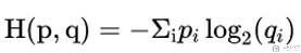
其中:

• p(真实的分布)，在实际中也就是 0 和 1，是正确的 label 就是 1，否则就是 0；
• q(预测的概率)，模型给出的概率（经过 softmax），都是介于 0-1 之间的数字；

因为 q 是介于 0-1 之间的数字，所以经过 log 之后为负数，然后前面又加了一个负号。如果对正确标签给出的概率越大，那个这个值就会越小（例如 log(0.5)=-0.69，log(0.99)=-0.01）。于是整个的 loss 可以定义为下面的样子：

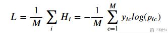
其中：

• M 为总的数据的数量；
• y 是实际标签, 为 one-hot 编码；
• p 为模型输出的概率；

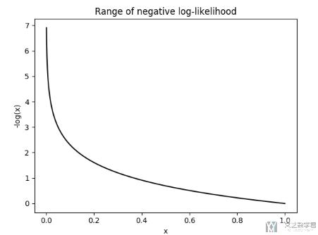
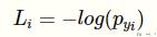
在实际中，因为 y 只有 0 和 1 两种不同的取值，所以 negative log-likelihood 可以化简为下面的式子：

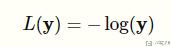
我们画出上面的 L 关于不同输入的图像，可以看到当概率很小的时候，L 会很大；当概率大的时候，L 会很小。也就是说，当网络给正确的结果一个很低的置信度(confidence)的时候, 此时 L 很大（我们希望 L 越小越好）：

还是上面的例子，在计算完 softmax 之后，我们计算 NLLLoss。下图中红色的表示正确的是哪一类：

于是，我们使用上面的交叉熵来衡量上面的模型一和模型二。需要注意的是, 在 Pytorch 中，有一个函数是 NLLLoss (negative log likelihood loss)，但是他并没有计算 log，这个名字起的很奇怪。关于 NLLLoss 的介绍可以查看连接， PyTorch中交叉熵的计算-CrossEntropyLoss介绍

所以，在 Pytorch，多分类的 loss 我们会使用 nn.CrossEntropyLoss()，这里面包含了 Logsoftmax+NLLLoss，他把 Log 的计算和 sotfmax 和在了一起。

我们在这里就自己手动计算 log，再使用 NLLLoss 来测试一下上面两个模型的好坏。(我们认为是模型二比模型一要好)，注意下面的代码，我们对概率值手动计算了 log：

可以看到模型一的 loss 比模型二的要大，说明模型二比较好。

关于 Sotfmax 和 NLLLoss 的数学推导

数学推导

上面我们直观的了解了一下 Softamx 和 NLLLoss 的相关内容，这里我们来计算一下他们的导数，更进一步说明这样做的好处。(这一部分的数学推导来自，Understanding softmax and the negative log-likelihood)

首先重写一下关于 softmax 的函数：

接着是 negative log-likelihood 的函数:

我们是要计算 L 关于 f 的导数，我们可以使用链式法则进行如下的展开：

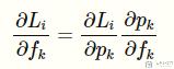
这样就分为了两个部分，我们首先看一下前面一部分：

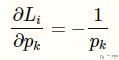
接着我们来计算第二部分。在计算之前，复习一下除法的求导公式：

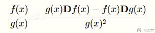
按照上面的方式，对第二部分的式子进行求导：

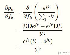
继续对上面的式子进行化简：

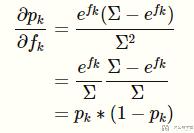
最后我们将第一部分和第二部分结合起来，总的导数为：

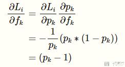
可以看到最终的导数很简单，这也就是为什么通常情况下，我们都是将 softmax 和 negative log likelihood 合起来一起用的，也就是 Pytorch 中的 CrossEntropyLoss。

下面我们使用 CrossEntropyLoss 来做一下实验，看一下导数是不是和我们推导的是一样的。

使用 CorssEntropyLoss 进行实验

我们还是使用之前的实验数据来进行模拟。下面我们使用了sum，也就是将每一条数据的 loss 进行求和。

我们看一下 X 进行 softmax 之后的结果：

可以看到和上面图上是一样的。下面我们再来确认一下上面 loss 的计算。为了自己手动计算 loss。我们需要对 Softmax 的结果求 log。

于是 loss 的计算也就变成了, loss=0.3490+0.0206+0.7177=1.0873。

上面我们再次确认了 CrossEntropyLoss 是如何进行计算的。下面我们确认上面的求导公式。我们首先进行反向传播，计算X的梯度。

三个负数的值(对应第一条数据的第一个, 第二条数据的第三个, 第三条数据的第二个),  也就是对应label=1的数据, 都是通过(p-1)计算得到的, 其他的都是p (因为y=0, 所以其实在计算NLL Loss的时候没有参与运算).

下面是按照上面的公式推导出来的导数，看到和上面解释的是一样的：

于是, 使用 CrossEntropyLoss 的总的一个流程如下图所示: